Pytorch基础

本篇是对Pytorch基础使用的学习，主要基于B站小土堆的https://www.bilibili.com/video/BV1hE411t7RN/以及Gemini的帮助，除实践外也包含了一些深度学习模型的原理

Dataset

An abstract class representing a Dataset.

All datasets that represent a map from keys to data samples should subclass it. All subclasses should overwrite __getitem__, supporting fetching a data sample for a given key. Subclasses could also optionally overwrite __len__, which is expected to return the size of the dataset by many ~torch.utils.data.Sampler implementations and the default options of ~torch.utils.data.DataLoader. Subclasses could also optionally implement __getitems__, for speedup batched samples loading. This method accepts list of indices of samples of batch and returns list of samples.

note

~torch.utils.data.DataLoader by default constructs an index sampler that yields integral indices. To make it work with a map-style dataset with non-integral indices/keys, a custom sampler must be provided.

一个表示数据集的抽象类。

所有实现从键（keys）到数据样本（data samples）映射的数据集都应该继承这个类。所有子类都必须重写 __getitem__ 方法，以支持根据给定的键获取数据样本。子类也可以选择性地重写 __len__ 方法，许多 ~torch.utils.data.Sampler 实现和 ~torch.utils.data.DataLoader 的默认选项都需要通过这个方法返回数据集的大小。子类还可以选择性地实现 __getitems__ 方法，以加速批量样本的加载。此方法接受批处理样本的索引列表，并返回样本列表。

注意

默认情况下，~torch.utils.data.DataLoader 会构造一个生成整数索引的采样器。要让其与非整数索引/键的映射式数据集一起工作，必须提供自定义的采样器。

自定义Dataset

那么在实际的使用中，比如有一个数据集（我们拿之前用过的fer2013来举例）：

先定义一个数据类继承Dataset，定义__init__()

from torch.utils.data import Dataset
import os
class MyData(Dataset):
    def __init__(self, root_dir, label_dir):
        self.root_dir = root_dir # 如 fer2013/test
        self.label_dir = label_dir # 如 angry
        self.path = os.path.join(self.root_dir, self.label_dir) # 路径合并函数 解决跨系统的文件路径问题
        self.img_path = os.listdir(self.path) # 如angry文件夹下，所有图片名的string list

重写__getitem()

def __getitem__(self, index):
        img_name = self.img_path[index]
        img_item_path = os.path.join(self.root_dir, self.label_dir, img_name) # 拼接出具体的某一个图片的路径
        img = Image.open(img_item_path)
        label = self.label_dir
        return img, label # 返回数据集中的一个对象（图片）及其类型

重写__len()__

def __len__(self):
        return len(self.img_path)

定义示例

root_dir = "fer2013/train"
angry_label_dir = "angry"
angry_dataset = MyData(root_dir, angry_label_dir)

Dataset合并

disguest_label_dir = "disguest"
disgust_dataset = MyData(root_dir, disguest_label_dir)

train_dataset = angry_dataset + disgust_dataset # '+'

TensorBoard

SummaryWriter

创建日志目录
初始化Writer对象
生成事件文件
- 这个文件才是真正的数据库(events.out…)当后续调用 writer.add_scalar 时，数据并不是直接画在屏幕上，而是被追加写进这个文件里。
- 当你执行完相应代码，运行 tensorboard --logdir=logs 时，TensorBoard 的后端服务器就会去读取这个文件里的内容，并在浏览器里渲染成图表。

from torch.utils.tensorboard import SummaryWriter

writer  = SummaryWriter("logs") # 这行代码会在你的项目根目录下创建一个名为"logs"的文件夹

需注意，每次实验可以用不同的文件夹来记录数据，比如writer = SummaryWriter("logs/lr0.01_batch32")修改了学习率后writer = SummaryWriter("logs/lr0.001_batch32")

add_scalar()

绘图函数add_scalar()

(method) def add_scalar(
    tag: Any,
    scalar_value: Any, # 对应图像的y轴
    global_step: Any | None = None, # 对应图像的x轴
    walltime: Any | None = None,
    new_style: bool = False,
    double_precision: bool = False
) -> None

``` 例 ```

for i in range(100):
    writer.add_scalar("y=2x", 2*i, i)
writer.close()

add_image()

查看图片函数add_image()

(method) def add_image(
    tag: Any,
    img_tensor: Any,
    global_step: Any | None = None,
    walltime: Any | None = None,
    dataformats: str = "CHW"
) -> None

要注意参数的类型要求：img_tensor (torch.Tensor, numpy.ndarray, or string/blobname): Image data，所以要将PIL类型的图片进行转换，比如用numpy来转换。以及数据的shape要求： Tensor with :math:(1, H, W), :math:(H, W), :math:(H, W, 3) is also suitable as long as corresponding dataformats argument is passed, e.g. CHW, HWC, HW. 即三种图片数据的格式，其通道数、高度、宽度的顺序不同。

img = Image.open(image_path)
img_array = np.array(img)
print(f"图像形状: {img_array.shape}")
writer.add_image("test",img_array,1,dataformats='HW') # 由.shape可得
writer.close()

add_graph()

常见的Transforms

下面基本都是对图像的处理方法

ToTensor

Convert a PIL Image or ndarray to tensor and scale the values accordingly.

This transform does not support torchscript.

Converts a PIL Image or numpy.ndarray (H x W x C) in the range [0, 255] to a torch.FloatTensor of shape (C x H x W) in the range [0.0, 1.0] if the PIL Image belongs to one of the modes (L, LA, P, I, F, RGB, YCbCr, RGBA, CMYK, 1) or if the numpy.ndarray has dtype = np.uint8

In the other cases, tensors are returned without scaling.

note

Because the input image is scaled to [0.0, 1.0], this transformation should not be used when transforming target image masks. See the [references](vscode-file://vscode-app/d:/Microsoft VS Code/resources/app/out/vs/code/electron-browser/workbench/workbench.html) for implementing the transforms for image masks.
将PIL图片转为torch类型，如torch.Size([1, 48, 48])

trans_totensor = transforms.ToTensor()
img_tensor = trans_totensor(img)
print(img_tensor.shape)
writer.add_image("ToTensor",img_tensor)
writer.close()

Normalize

Normalize a tensor image with mean and standard deviation.

This transform does not support PIL Image.

Given mean: (mean[1],...,mean[n]) and std: (std[1],..,std[n]) for n

channels, this transform will normalize each channel of the input

torch.*Tensor i.e.,

output[channel] = (input[channel] - mean[channel]) / std[channel]

note:

This transform acts out of place, i.e., it does not mutate the input tensor.

Args:

mean (sequence): Sequence of means for each channel.

std (sequence): Sequence of standard deviations for each channel.

inplace(bool,optional): Bool to make this operation in-place.

Normailize 的数学原理是：

output = \frac{input-mean}{std}

参数mean影响的是“中心位置”，在ToTensor之后，像素值在 $[0, 1]$ 之间，中心大约在 $0.5$ ，如mean = 0.5，那么减去 $0.5$ 后，数据的中心变成了 $0$ 。原本 $[0, 1]$ 的范围变成了 $[-0.5, 0.5]$
参数std影响的是“缩放幅度”，如std = 0.5，那么就是将数据范围再除以 $0.5$ ，最终范围从 $[-0.5, 0.5]$ 变成了 $[-1, 1]$

Resize

Resize the input image to the given size.

If the image is torch Tensor, it is expected

to have […, H, W] shape, where … means a maximum of two leading dimensions

Args:

size (sequence or int): Desired output size. If size is a sequence like

(h, w), output size will be matched to this. If size is an int,

smaller edge of the image will be matched to this number.

i.e, if height > width, then image will be rescaled to

(size * height / width, size).

resize()支持PIL和Tensor两种图片格式，如果是 Tensor，期望形状为 [..., H, W]。这里的 ... 表示它可以处理 [C, H, W]（单张图）或 [B, C, H, W]（一个 Batch 的图）
参数size需注意写成序列形式，如resize((512, 512))，而如果只输入一个参数，如resize(512)，那么图片短边会变为512，而长边会按比例改变

print(img.size)
trans_resize = transforms.Resize((224,224))
img_resize = trans_resize(img)
print(img_resize)

Compse

Composes several transforms together. This transform does not support torchscript.

Please, see the note below.

Args:

transforms (list of Transform objects): list of transforms to compose.

compse()操作是对各种transforms操作的流水线类
在深度学习中，图片通常需要经过一系列的固定步骤（比如：缩放 -> 转为 Tensor -> 归一化）。如果不用 Compose，你每一张图都要手动调用多个函数，代码会非常冗余
compse()的参数类型是一个列表，操作是按顺序执行的，所以前一个操作输出的数据类型必须能作为下一个操作的输入。

from torchvision import transforms
# 定义训练集的预处理
train_transform = transforms.Compose([
    transforms.Resize((224, 224)),           # VGG16标准输入是224x224
    transforms.RandomHorizontalFlip(),       # 数据增强：随机水平翻转
    transforms.ToTensor(),                   # 归一化到 [0.0, 1.0]
    transforms.Normalize([0.5], [0.5])       # 标准化到 [-1.0, 1.0]
])
img_tensor = train_transform(img)

Pytorch数据集使用

例如，我们要导入视觉学习的数据集，可以直接在程序中进行数据集的下载

import torchvision

train_set = torchvision.datasets.CIFAR10(root="./dataset...", train=True, download=True)

test_set = torchvision.datasets.CIFAR10(root="./dataset...", train=false, download=True)

root参数表示数据集存放的位置，train参数表示数据集是否用来训练，download参数表示是否下载到本地（会生成一个下载链接）
具体的参数设置，每个数据集都可能有所区别…
如果是下载完成到本地的数据集，可以将其复制到项目目录的dataset文件夹下，再运行程序即可节省下载的时间

print(test_set.classes) # 可以看到测试数据集的所有类别

img, target = test_set[0]
print(img)
print(target)
print(test_set.classes[target]) # 输出测试集第一个元素对应的类别

DataLoader

Data loader combines a dataset and a sampler, and provides an iterable over the given dataset.

The :class:~torch.utils.data.DataLoader supports both map-style and

iterable-style datasets with single- or multi-process loading, customizing

loading order and optional automatic batching (collation) and memory pinning.

在训练模型时，不能一次性把数据集中的大量数据塞进内存。DataLoader实现了：

Batching（批处理）： 把图片打包成一组组（Batch）。
Shuffling（打乱）： 每一轮训练（Epoch）开始时随机洗牌，防止模型死记硬背数据顺序。
Parallel Computing（并行加载）： 利用多核 CPU 提前准备下一批数据，不让 GPU 等待。

参数名	常用取值	作用描述
dataset	自定义 Dataset	必填。告诉 DataLoader 从哪个“仓库”取数据。
batch_size	16, 32, 64…	每批装载的数量。越大训练越快，但越占显存。在 FER 表情识别中，32 或 64 是常用数值。
shuffle	`True` / `False`	是否打乱顺序。训练集通常设为 `True`（增加随机性）；测试集通常设为 `False`。
num_workers	0, 2, 4, 8…	多进程加载。 `0` 表示只用主进程（慢）。增加数值可以加快读取速度。建议：设为 CPU 核心数的一半。
drop_last	`True` / `False`	丢弃最后多余的数据。比如有 100 张图，`batch_size=32`。最后剩 4 张不够一包，设为 `True` 就会把这 4 张扔掉，确保每个 Batch 大小一致。
pin_memory	`True`	内存锁页。如果你用 GPU 训练，设为 `True` 可以加快数据从内存传输到显存的速度。

例如，我们用DataLoader处理CIFAR10中的数据

test_data = torchvision.datasets.CIFAR10("./dataset", train=False, transform=torchvision.transforms.ToTensor(), download=True)

test_loader = DataLoader(dataset=test_data, batch_size=4, shuffle=True, num_workers=0, drop_last=False)

结合循环和tensorboard，输出每一个epoch中每一step用到的图片
下面代码中step + epoch * len(test_loader)是使用了全局步长，也可以不这样写，而是把每个epoch来当作一组

writer = SummaryWriter("dataloader")
for epoch in range(2):
    step = 0
    for data in test_loader:
        imgs, targets = data
        writer.add_images("test_data_batch", imgs, step + epoch * len(test_loader))
        step = step + 1
writer.close()

nn.Module

Base class for all neural network modules.

Your models should also subclass this class.

Modules can also contain other Modules, allowing to nest them in a tree structure.

在 PyTorch 中，无论是简单的线性层，还是复杂的 VGG16 或 Transformer，本质上都是一个 nn.Module。它是所有神经网络模块的基类
nn.Module 支持嵌套，当你对大模型调用 model.to("cuda") 时，PyTorch 会顺着这棵“树”，自动把里面所有的子层都搬到 GPU 上。
只要在 __init__ 中把一个层赋值给 self.xxx，PyTorch 就会自动识别出其中的权重 (Weights) 和 偏置 (Bias)，并将它们加入到待优化的参数列表中。

编写一个nn.Module子类时，必须重写__init()__和forward()

__init(self)__
- 在这里定义网络层（卷积、池化、全连接等）。
- 必须调用 super().__init__()。这行代码的作用是初始化父类的属性，如果没有它，PyTorch 就没法自动追踪定义的层，模型也就无法训练。
forward(self, x)
- 定义数据的流向。图片进去后，先过哪一层，再过哪一层。
- 不需要手动调用 forward，只需要运行 model(input)，PyTorch 会自动触发 forward。

import torch
from torch import nn

class myModule(nn.Module):
    def __init__(self):
        super().__init__()

    def forward(self, input):
        output = input + 1 # 简单地将输出 +1 再输出
        return output

卷积 Conv

\text{out}(N_i, C_{\text{out}_j}) = \text{bias}(C_{\text{out}_j}) + \sum_{k = 0}^{C_{\text{in}} - 1} \text{weight}(C_{\text{out}_j}, k) \star \text{input}(N_i, k)

卷积动画页面：conv_arithmetic/README.md at master · vdumoulin/conv_arithmetic

参数	含义	作用
in_channels	输入通道数	彩色图通常为 3 (RGB)，灰度图为 1。
out_channels	输出通道数	卷积核的数量。有多少个核，输出就有多少层特征图。
kernel_size	卷积核大小	提取特征的“窗口”大小。常用 3 或 5（VGG 常用 3）。
stride	步长	窗口滑动的跨度。默认为 1。步长越大，输出图片越小。
padding	填充	在图片四周补 0。`'same'` 保持大小不变，`'valid'` 则不补。
dilation	空洞卷积	卷积核点之间的间距。用于扩大感受野（不用增加参数量）。
bias	偏置	是否在结果上加一个常数偏移。默认开启。

卷积的Padding（边界扩充）参数很重要，如果周围不补零，那么卷积会导致图像尺寸越来越小
形状计算公式：

H_{out} = \left\lfloor\frac{H_{in} + 2 \times \text{padding}[0] - \text{dilation}[0] \times (\text{kernel_size}[0] - 1) - 1}{\text{stride}[0]} + 1\right\rfloor

$W_{out}$ 计算同理

dataset = torchvision.datasets.CIFAR10("./dataset",train = False, transform=torchvision.transforms.ToTensor(),download=True)
dataloader = DataLoader(dataset, batch_size=64)

class myModule(nn.Module):
    def __init__(self):
        super().__init__()
        self.conv1 = Conv2d(in_channels=3,out_channels=6,kernel_size=3,stride=1,padding=0)

    def forward(self,x):
        x = self.conv1(x)
        return x

mymodule = myModule() # 模型实例化

step = 0
for data in dataloader:
    imgs, targets = data
    output = mymodule(imgs)
    print(imgs.shape)
    # torch.Size([64, 3, 32, 32])
    print(output.shape)
    # torch.Size([64, 6, 30, 30]) channel == 6 卷积后，channel数变化，不能直接输出图像

    step = step + 1

（最大）池化 MaxPool

最大池化的逻辑非常简单：在一个窗口（Kernel）范围内，只保留最大的那个值，剩下的全部扔掉
既保留输入特征，又减小了数据量，加快训练速度

参数	独特之处
kernel_size	窗口大小。常见是 `2`（即将 $2 \times 2$ 的区域合并）。
stride	默认值等于 kernel_size！这和卷积不同。如果 `kernel_size=2`，步长默认就是 `2`，这样窗口之间就不会重叠。
ceil_mode	非常重要。默认是 `False`（向下取整）。如果设为 `True`（向上取整），当窗口超出边界时，只要窗口内有数据，就会保留结果，而不是舍弃。
padding	填充。注意池化填充的是负无穷（ $-\infty$ ），这样是为了保证填充位不会被选为最大值。

input = torch.tensor([[1,2,0,3,1],
                     [0,1,2,3,1],
                     [1,2,1,0,0],
                     [5,2,3,1,1],
                     [2,1,0,1,1]], dtype=float)

input = torch.reshape(input,(-1,1,5,5))
print(input.shape)

class myMoudle(nn.Module):
    def __init__(self, *args, **kwargs):
        super(myMoudle, self).__init__()
        self.maxpool1 = MaxPool2d(kernel_size=3, ceil_mode=True) 
        '''
        ceil_mode = False 就表示只有当池化核遇到的尺寸是最大尺寸（如3x3）时
        才会取其池化的结果，否则相反
        '''
    def forward(self, input):
        output = self.maxpool1(input)
        return output
    
mymoudle = myMoudle()
output = mymoudle(input)
print(output)

torch.Size([1, 1, 5, 5])
tensor([[[[2., 3.],
          [5., 1.]]]], dtype=torch.float64)

损失函数与反向传播

损失函数用于计算实际输出与目标之间的差距，为反向传播、更新参数提供一定的依据。在分类任务中，常用交叉熵函数来计算误差，

loss_func = nn.CrossEntropyLoss()

优化器

torch.optim — PyTorch 2.10 documentation

示例代码：

for input, target in dataset:
    optimizer.zero_grad() # 梯度清零
    output = model(input)
    loss = loss_fn(output, target) # 调用损失函数
    loss.backward() # 反向传播
    optimizer.step()

Pytorch实战：CIFAR10

针对CIFAR10图像数据集的简单分类模型实战

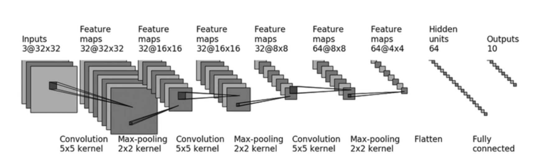
首先了解Sequential，nn.Sequential 是 nn.Module 的一个特殊子类，它的作用是自动完成 forward 逻辑。注意：其中每一个参数都是某层的类，所以要写逗号。Sequential既简化了模型定义，也简化了forward()。

class CIFAR10_Simple(nn.Module):
    def __init__(self, *args, **kwargs):
        super(CIFAR10_Simple, self).__init__(*args, **kwargs)
        self.conv1 = Conv2d(in_channels=3, out_channels=32, kernel_size=5, padding=2)
        '''
        参数padding的数值可以从想象图像得到：5x5的卷积核，当中心在图像的(0,0)，那么卷积核是扩展出去2格的。上面是简单判断的方法，实际应该用尺寸计算公式来代入计算（参考“Conv卷积”节内容）
        '''
        self.model_s = Sequential(
            Conv2d(in_channels=3, out_channels=32, kernel_size=5, padding=2),
            nn.ReLU(),
            MaxPool2d(kernel_size=2),
            Conv2d(in_channels=32, out_channels=32, kernel_size=5, padding=2),
            nn.ReLU(),
            MaxPool2d(2),
            Conv2d(32,64,5,padding=2),
            nn.ReLU(),
            MaxPool2d(2),
            Flatten(),
            Linear(1024, 64),
            nn.ReLU(),
            Linear(64, 10)
        )

    def forward(self, x):
        '''
        x = self.conv1(x)
        x = self.maxpool1(x)
        x = self.conv2(x)
        x = self.maxpool2(x)
        x = self.conv3(x)
        x = self.maxpool3(x)
        x = self.flatten(x)
        x = self.linear1(x)
        x = self.linear2(x)
        '''
        x = self.model_s(x)
        return x

在搭建模型前，先设置DataLoader处理数据集
- 分别设置好train_data和test_data

dataset_transfrom = tf.Compose([tf.ToTensor(),tf.Normalize((0.5,0.5,0.5),(0.5,0.5,0.5))])
train_data = torchvision.datasets.CIFAR10("./dataset", transform=dataset_transfrom, download=True)
test_data = torchvision.datasets.CIFAR10("./dataset", train=False, transform=dataset_transfrom, download=True)
# --------
train_loader = DataLoader(dataset=train_data, batch_size=64, shuffle=True, drop_last=True)
test_loader = DataLoader(dataset=test_data, batch_size=64, shuffle=True, drop_last=True)

搭建好模型后，简单测试输出尺寸是否符合要求

cifar = CIFAR10_Simple()
print(cifar)
input = torch.ones((64, 3, 32, 32)) # 同数据集图片尺寸的测试
output = cifar(input)
print(output.shape)

训练前的基本设置
- 定义TensorBoard的writer
- 设置device调用显卡加速训练
- 实例化训练模型
- 定义损失函数
- 设置优化器

writer = SummaryWriter("./logs")
writer.add_graph(cifar, input)
device = torch.device("cuda" if torch.cuda.is_available() else "cpu")
model = CIFAR10_Simple().to(device)
loss_func = nn.CrossEntropyLoss() # 交叉熵损失函数
optim = torch.optim.SGD(cifar.parameters(), lr=0.01) # 学习率

训练部分
- 优化器的定式代码
- 记录训练损失

total_step = 0
for epoch in range(10):
    # --- 训练部分 ---
    model.train()
    for data in train_loader:
        imgs, targets = data
        outputs = model(imgs.to(device))
        loss = loss_func(outputs, targets.to(device))
        
        optim.zero_grad()
        loss.backward()
        optim.step()
        
        # 记录训练损失
        writer.add_scalar("Train_Loss", loss.item(), total_step)
        total_step += 1

评估部分
- 每个epoch执行一次
- with torch.no_grad()：关闭梯度记录
- 统计性能指标

model.eval()
    total_test_loss = 0
    total_accuracy = 0
    with torch.no_grad(): # 测试时不需要计算梯度，节省性能
        for data in test_loader:
            imgs, targets = data
            imgs, targets = imgs.to(device), targets.to(device)
            outputs = model(imgs)
            
            # 计算总损失
            loss = loss_func(outputs, targets)
            total_test_loss += loss.item()
            
            # 计算准确率：argmax(1) 找到概率最大的类别索引
            accuracy = (outputs.argmax(1) == targets).sum()
            total_accuracy += accuracy

可视化

# 输出到 TensorBoard
    writer.add_scalar("Test_Loss", total_test_loss / len(test_loader), epoch)
    writer.add_scalar("Test_Accuracy", total_accuracy / len(test_data), epoch)
    
    print(f"Epoch {epoch+1} 结束，准确率: {total_accuracy / len(test_data)}")

writer.close()