cs224n

Intro

本篇是对Stanford CS 224N | Natural Language Processing with Deep Learning (Spring 2024)这门课程的学习笔记。关于这门课的内容，总结如下：

• 词向量、RNN、LSTM、Seq2Seq 模型、机器翻译、注意力机制、Transformer 等等

What is this course about?

Natural language processing (NLP) or computational linguistics is one of the most important technologies of the information age. Applications of NLP are everywhere because people communicate almost everything in language: web search, advertising, emails, customer service, language translation, virtual agents, medical reports, politics, etc. In the 2010s, deep learning (or neural network) approaches obtained very high performance across many different NLP tasks, using single end-to-end neural models that did not require traditional, task-specific feature engineering. In the 2020s amazing further progress was made through the scaling of Large Language Models, such as ChatGPT. In this course, students will gain a thorough introduction to both the basics of Deep Learning for NLP and the latest cutting-edge research on Large Language Models (LLMs). Through lectures, assignments and a final project, students will learn the necessary skills to design, implement, and understand their own neural network models, using the Pytorch framework.

Word Vectors

$ vector(”King”)- vector(”Man”) + vector(”Woman”) $ results in a vector that is closest to the vector representation of the word Queen

How do we have usable meaning in a computer?

Slides里介绍了几种方式：

• WordNet
• one-hot vectors
• word vectors

那么前两种都有其现实意义，但也有明显的弊端。

• WordNet，完全靠synonum sets和hypernyms sets来确定词汇间的关系、构造复杂、无法及时吸收新词汇…

• one-hot vectors给每个词都设置了symbol，尽管是用数字表达，但是相近的词之间在数学上没有联系（向量的点积为0）

那么下面就引出了一句名言：“You shall know a word by the company it keeps”

以及word vectors的思想，将词汇归一化到一个向量中，虽然每个词汇有多个词义，但其分布却近似是其多个词义的平均，并用点积来确定词向量间的相关性。

Word2vec

original word2vec paper

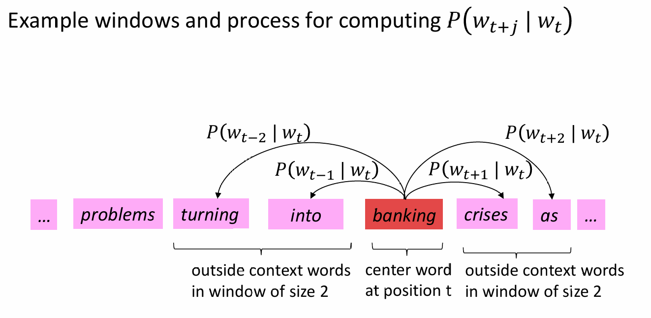
Word2vec很好地反映了word vectors的思想，计算中心词和相邻词的相似度，确定其概率分布：

• We have a large corpus (“body”) of text: a long list of words
• Every word in a fixed vocabulary is represented by a vector
• Go through each position t in the text, which has a center word c and context (“outside”) words o
• Use the similarity of the word vectors for c and o to calculate the probability of o given c (or vice versa)
• Keep adjusting the word vectors to maximize this probability

Objective Function

那么如何计算其似然程度(Likelihood)呢，For each position = $t=1,......,T$, predict context words within a window of fixed size $m$, given center word $w_t$. Data likelihood :

$$L(\theta) = \prod_{t=1}^{T} \prod_{\substack{-m \le j \le m \\ j \neq 0}} P(w_{t+j} \mid w_t; \theta)$$

为减小数据复杂程度，及方便计算机处理，优化上公式，对其进行平均负对数似然操作，The objective function $J(\theta)$ is the (average) negative log likelihood:

$$J(\theta) = -\frac{1}{T} \log L(\theta) = -\frac{1}{T} \sum_{t=1}^{T} \sum_{substack{-m \le j \le m \\ j \neq 0}} \log P(w_{t+j} \mid w_t; \theta)$$

最小化 $J(\theta)$ 等价于 最大化预测准确率。

Prediction Function

$$P(o \mid c) = \frac{\exp(u_o^T v_c)}{\sum_{w \in V} \exp(u_w^T v_c)}$$

1. $u_o^T v_c$ : 点积越大，代表这两个词在向量空间中的位置越接近，即语义相关性越高。
   Dot product compares similarity of o and c. $u^T v = u \cdot v = \sum_{i=1}^{n} u_i v_i$ Larger dot product = larger probability.
2. $\exp()$ : 将任何实数映射为正数。由于指数函数的增长特性，它会放大较大点积的影响，使相关性高的词获得更高的权重。
3. ${\sum_{w \in V} \exp(u_w^T v_c)}$ : 分母是对词汇表$V$中所有可能的词进行求和。这一步确保了所有可能输出的概率之和等于 1，从而构成一个标准的概率分布。

这也是对Softmax Function的应用

$$\text{softmax}(x_i) = \frac{\exp(x_i)}{\sum_{j=1}^{n} \exp(x_j)} = p_i$$

• Softmax 函数将任意值 $x_i$ 映射为一个概率分布 $p_i$。
• “max”：因为它会放大最大值 $x_i$ 对应的概率，使大的更大。
• “soft”：因为它仍然会给较小的 $x_i$ 分配一些概率。

To Train the Model

To train a model, we gradually adjust parameters to minimize a loss.

$$\theta = \begin{bmatrix} v_{aardvark} \\ v_a \\ \vdots \\ v_{zebra} \\ u_{aardvark} \\ u_a \\ \vdots \\ u_{zebra} \end{bmatrix} \in \mathbb{R}^{2dV}$$

• 如果词向量维度为 $d$，词汇量为 $V$，则总参数量为 $2dV$。

• 每个单词有两个向量，$\theta$ 包含了词汇表中所有单词的两种向量表示（中心词向量 $v$ 和背景词向量 $u$）。

• 计算所有参数的梯度，以优化模型

梯度公式就是对Softmax Function的求偏导，数学过程如下：

1. 初始损失函数 (单词对的负对数似然)
   这是针对一个中心词 $c$ 和一个背景词 $o$ 的基本损失定义：

   $$\text{Loss} = -\log P(o \mid c)$$

2. 代入Softmax定义展开
   将 $P(o|c)$ 的公式代入，利用对数性质将除法化为减法：

   $$\text{Loss} = -\log \left( \frac{\exp(u_o^T v_c)}{\sum_{w \in V} \exp(u_w^T v_c)} \right) = -u_o^T v_c + \log \sum_{w \in V} \exp(u_w^T v_c)$$

3. 第一部分求导
   对点积项关于中心词向量 $v_c$ 求偏导：

   $$\frac{\partial}{\partial v_c} (u_o^T v_c) = u_o$$

4. 第二部分求导
   利用链式法则对 $\log \sum \exp(\dots)$ 形式进行求导：

   $$\frac{\partial}{\partial v_c} \log \sum_{w \in V} \exp(u_w^T v_c) = \frac{1}{\sum_{w \in V} \exp(u_w^T v_c)} \cdot \sum_{x \in V} \left[ \exp(u_x^T v_c) \cdot u_x \right]$$

5. 转化为概率期望形式
   将上一步的结果重新组合，提取出原始的概率项 $P(x|c)$：

   $$\sum_{x \in V} \left[ \frac{\exp(u_x^T v_c)}{\sum_{w \in V} \exp(u_w^T v_c)} \right] u_x = \sum_{x \in V} P(x \mid c) u_x$$

6. 最终梯度公式
   将两部分合并，得到最终用于更新 $v_c$ 的梯度：

   $$\frac{\partial \text{Loss}}{\partial v_c} = -u_o + \sum_{x \in V} P(x \mid c) u_x$$

Gradient Descent

梯度下降更新方程 (矩阵形式)

$$\theta^{new} = \theta^{old} - \alpha \nabla_{\theta} J(\theta)$$

梯度下降更新方程 (单个参数形式)

$$\theta_j^{new} = \theta_j^{old} - \alpha \frac{\partial}{\partial \theta_j^{old}} J(\theta)$$

• $\alpha$ (alpha): 步长或学习率（step size / learning rate）。

但是实际应用并非上面的方法，而是用随机梯度下降，(Stochastic Gradient Descent, SGD)

• 目标函数 $J(\theta)$ 是语料库中所有窗口的函数。如果每次更新都要计算整个语料库的梯度 $\nabla_{\theta} J(\theta)$，计算成本极其昂贵，在进行单次更新前需要等待极长时间。
• SGD不再计算整个语料库，而是通过重复采样窗口，每处理一个（或一小批）窗口就更新一次参数。

Skip-gram Model with Negative Sampling

negative sampling paper

$$P(o\mid c)=\frac{\exp(u_x^T v_c)}{\sum_{w \in V} \exp(u_w^T v_c)}$$

采用最传统的方法计算概率时，即softmax，它的分母是全部词的叠加，计算量太大

而Skip-gram Model with Negative Sampling不需计算所有可能的词，而是训练一些逻辑回归，更偏好实际的上下文而非随机的上下文，实际上会选K个负样本，计算量就变为了$O(K)$

$$J_{neg-sample}(u_o, v_c, U) = -\log \sigma(u_o^T v_c) - \sum_{k \in \{K \text{ sampled indices}\}} \log \sigma(-u_k^T v_c)$$

其中，$\sigma(x)=\frac{1}{1+e^{-x}}$即sigmoid函数，使符合的结果概率接近于1，而不符合的则接近于0

但这又会导致低频词，如"zebra"的概率过低，而像"the"这样的词则概率较高，所以给公式加上$3/4$次方：

$$P(W)=U(W)^{3/4}/Z$$

来提高低频词的概率。

---

GloVe

original GloVe papar (Global Vectors for Word Representation)

Co-occurrence Martix

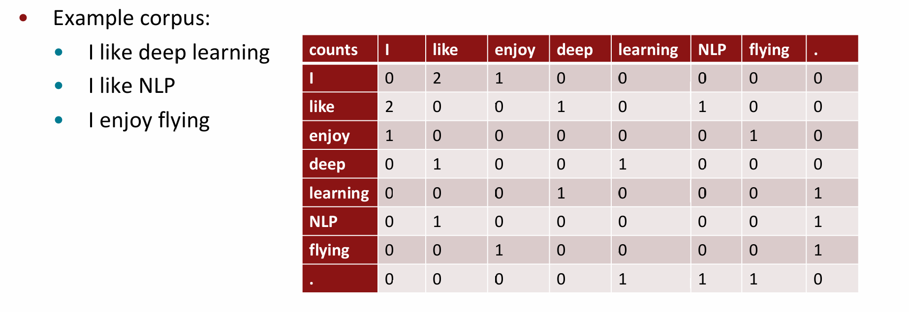
构建共现矩阵的方法非常简单，首先设定窗口长度，然后对在窗口长度内出现的共现词频率进行计数，一个简单的例子如上图（窗口为1，仅算相邻词）。但是：

• 词向量维度会随着语料库中词汇的增多而大幅增加，这会导致所需存储空间增大，且矩阵会变得相当稀疏，基于此构建的模型鲁棒性较差；
• 功能词出现频次极高，但没有提供相应的信息；
• 没有反映出词距与词相关性之间的联系。

那么如何进行降维来优化？经典的方法是进行SVD矩阵分解（虽然问了AI也没明白原理，而且Assignment1中用一个sklearn的函数就解决了）

$$X = U \Sigma V^T$$

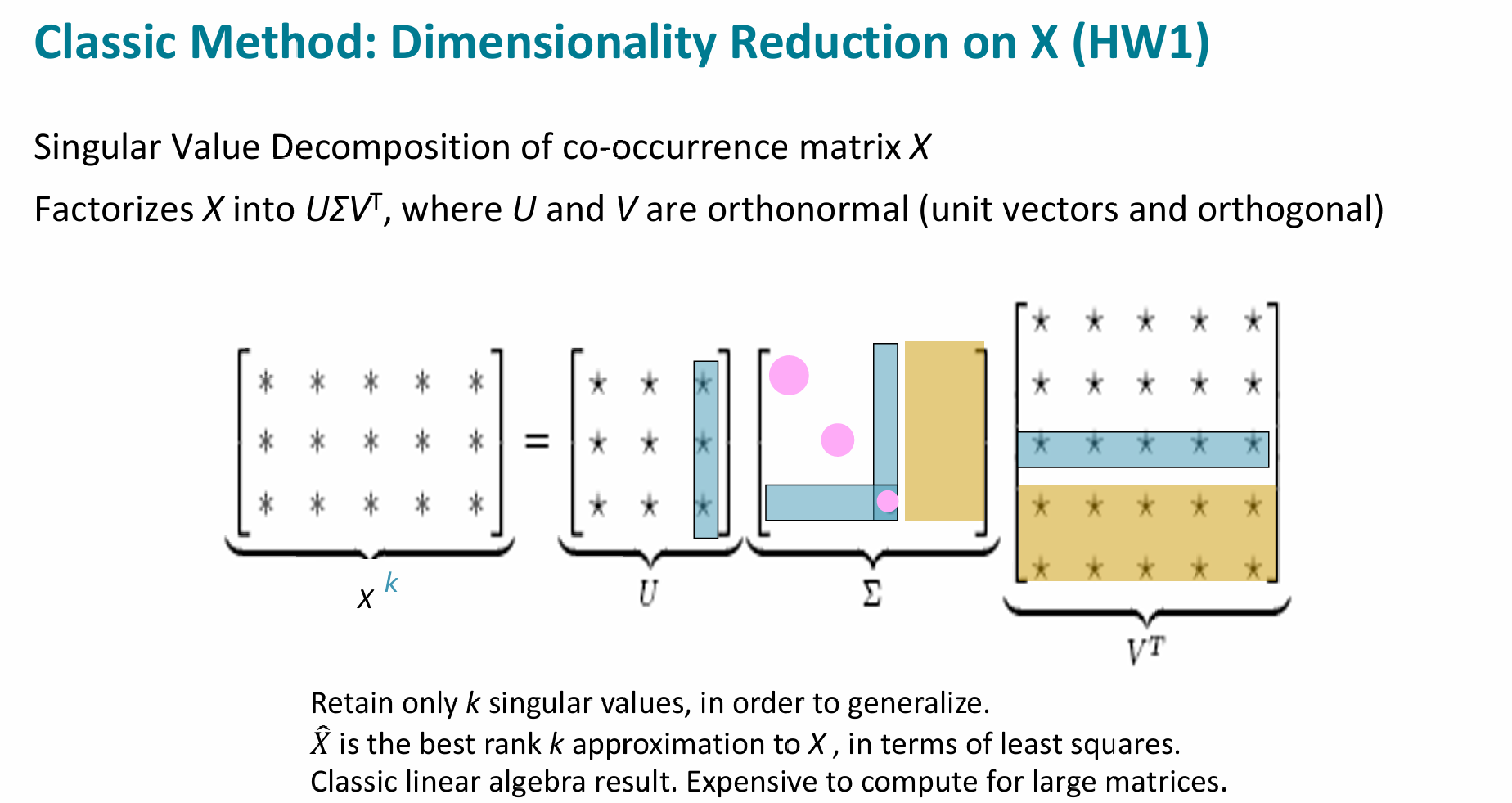
• $X$ (共现矩阵)：大小为 $|V| \times |V|$（词表大小）。每个元素 $X_{ij}$ 代表词 $i$ 和词 $j$ 在语料库中共同出现的次数。
• $U$ 和 $V$ (正交矩阵)：它们的列向量是相互正交的单位向量（Orthonormal）。在 NLP 中，$U$ 的每一行通常被视为该词的原始“嵌入”。
• $\Sigma$ (对角矩阵)：对角线上的值 $\sigma_1, \sigma_2, \dots$ 称为奇异值。它们按从大到小排列，代表了数据在对应维度上的重要程度（方差/信息量）。

那么降维便是将从共现矩阵得到的的，长度为$V$的词向量降维成长度为$K$的向量

真正编码语义的不是共现概率本身，而是共现概率的比值：

共现概率的比率可以编码语义成分，我们希望将它们作为线性语义成分捕捉在词向量空间中！

	$x = \text{solid}$	$x = \text{gas}$	$x = \text{water}$	$x = \text{fashion}$
$P(x\mid\text{ice})$	$1.9 \times 10^{-4}$	$6.6 \times 10^{-5}$	$3.0 \times 10^{-3}$	$1.7 \times 10^{-5}$
$P(x\mid\text{steam})$	$2.2 \times 10^{-5}$	$7.8 \times 10^{-4}$	$2.2 \times 10^{-3}$	$1.8 \times 10^{-5}$
$\dfrac{P(x\mid\text{ice})}{P(x\mid\text{steam})}$	$8.9$	$8.5 \times 10^{-2}$	$1.36$	$0.96$

Analogies

词向量虽然数学原理上很强大，但是其实际的类比(Analogy)场景却是有不少问题：

下例可见，是一个$woman+grandfather-man=?$的问题，那么显而易见且最有可能的结果就是grandmother，那么为何程序给出的另外几个，如granddaughter, mother之类，score也几乎一样很高呢？

# Run this cell to answer the analogy -- man : grandfather :: woman : x
pprint.pprint(wv_from_bin.most_similar(positive=['woman', 'grandfather'], negative=['man']))

[('grandmother', 0.7608445286750793),
 ('granddaughter', 0.7200808525085449),
 ('daughter', 0.7168302536010742),
 ('mother', 0.7151536345481873),
 ('niece', 0.7005682587623596),
 ('father', 0.6659888029098511),
 ('aunt', 0.6623409390449524),
 ('grandson', 0.6618767976760864),
 ('grandparents', 0.644661009311676),
 ('wife', 0.6445354223251343)]

虽说Assignment里没有标准答案，但是通过AI可以得知：这涉及到“语义聚类”

• 语义的“近邻效应”
  • 在向量空间中，逻辑相似的词通常会聚在一起形成一个“簇”。当你计算出 $\vec{w} + \vec{g} - \vec{m}$ 时，你实际上是在空间中定位了一个坐标点。
  • granddaughter 等同样具有“女性”和“亲属”属性，且在语料库中经常与 grandfather 或 grandmother 出现在相似的上下文。在向量维度上，它们在“亲属关系”这个维度上非常接近。
• 维度的“重叠性”
  • 词向量通常有几百个维度。虽然我们减去了 man 并加上了 grandfather，但这并不能完全抹除其他维度的相似性。
  • daughter、mother、grandmother 共享了绝大部分维度：[+女性]、[+人类]、[+亲属]。

下面的例子，属于"Incorrect Analogy"，我们来看易得答案为socks，但为何模型忽略了glove和hand，而输出了各种square的名词？显然和foot“脚”的释义无关，而是“英尺”的释义。

pprint.pprint(wv_from_bin.most_similar(positive=['foot', 'glove'], negative=['hand']))

[('45,000-square', 0.4922032654285431),
 ('15,000-square', 0.4649604558944702),
 ('10,000-square', 0.4544755816459656),
 ('6,000-square', 0.44975775480270386),
 ('3,500-square', 0.444133460521698),
 ('700-square', 0.44257497787475586),
 ('50,000-square', 0.4356396794319153),
 ('3,000-square', 0.43486514687538147),
 ('30,000-square', 0.4330596923828125),
 ('footed', 0.43236875534057617)]

• 语义多义性的干扰
  • 上面也提到，foot也是计量单位”英尺“的英文，和square组合是合理的
• 训练语料的偏见
  • 既然foot有多个释义，但输出却全是其“英尺”的意思，那么这可能体现了用来训练的语料中多是...square和foot相关联
• 词的选择
  • 即使输出全是...square，其score值也不过0.5，这不仅说明模型找不到强相关的词，而且说明了模型很可能没能理解glove与hand, foot的联系

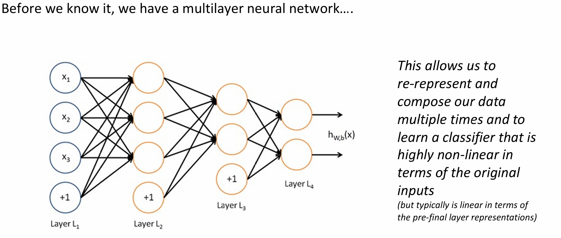
Neural Network

A neural network = running several logistic regressions at the same time.

CS231n Deep Learning on Network Architectures

CS231n Deep Learning for Computer Vision on Backprop

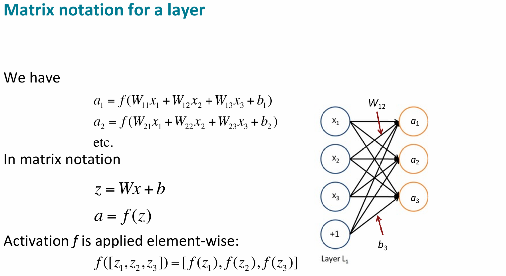
Structure

---

Non-linearities

为什么神经网络需要非线性(Non-linearities)？

• 核心观点：神经网络执行函数逼近，例如回归或分类。
  • 没有非线性：深度神经网络只能执行线性变换。
  • 多层失效：额外的层会被压缩成单个线性变换：$W_1 W_2 x = Wx$（即多层线性层等同于一层）。
  • 有了非线性：通过包含非线性的多层结构，网络可以逼近更复杂的函数！

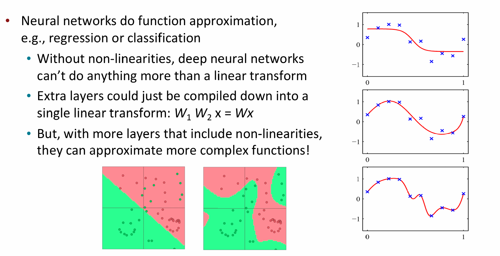
• 左下侧图对：左图显示线性分类（只能画直线），无法区分复杂的红绿点分布；右图显示非线性分类（可以画曲线），完美分割了数据。
• 右侧三张波形图：展示了随着函数复杂度的增加，只有非线性模型才能拟合这些起伏的蓝点（观测数据）。

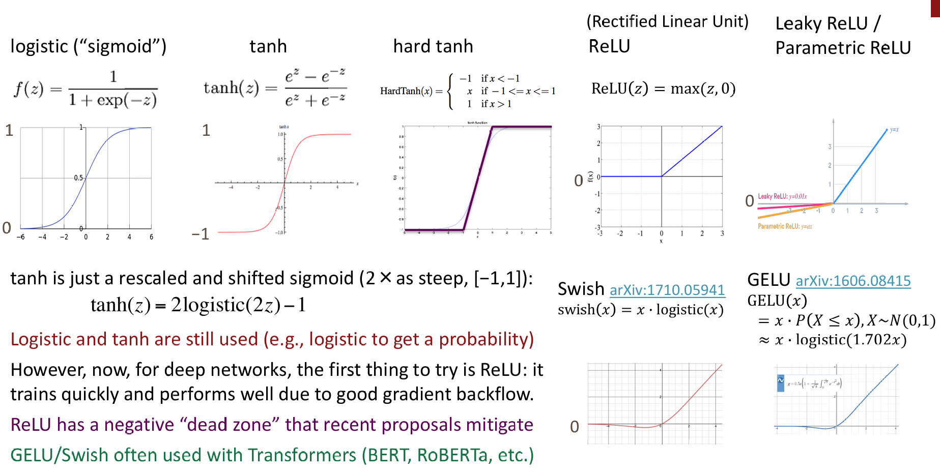
关于常用的非线性函数，在《智能计算系统》课上均有学习，不多赘述

---

Gradients

derivatives.pdf

梯度，简单地讲就是对变量的微积分，比如我们有：

$$f(x)=x^3$$

那么它的梯度就是：

$$\frac{df}{dx}=3x^2$$

当然，这只是个非常简单的例子，实际上是大规模的链式法则计算，对矩阵(Jacabian Matrix)进行梯度计算。

Chain Rule

在单变量微积分中，如果 $y = f(u)$ 且 $u = g(x)$，那么：

$$\frac{dy}{dx} = \frac{dy}{du} \cdot \frac{du}{dx}$$

但在神经网络中，每一层都是一个向量 $\mathbf{h,z} \in \mathbb{R}^n$。当我们将这个逻辑扩展到向量时，乘法就变成了矩阵乘法。

对于多个变量，应与Jacobians矩阵相乘：

假设有 $\mathbf h= f(z)$ 和 $\mathbf z=Wx+b$ ，下面的这些偏导数就是雅可比矩阵

$$\frac{\partial \mathbf{h}}{\partial \mathbf{x}} = \frac{\partial \mathbf{h}}{\partial \mathbf{z}} \frac{\partial \mathbf{z}}{\partial \mathbf{x}}$$

Matrix Calculus

由下式得，矩阵只有对角元素，其余部分均为0：

$$\begin{aligned} \left( \frac{\partial \mathbf{h}}{\partial \mathbf{z}} \right)_{ij} &= \frac{\partial h_i}{\partial z_j} = \frac{\partial}{\partial z_j} f(z_i) \quad && \text{definition of Jacobian} \\ &= \begin{cases} f'(z_i) & \text{if } i = j \\ 0 & \text{if otherwise} \end{cases} \quad && \text{regular 1-variable derivative} \end{aligned}$$

$$\frac{\partial \mathbf h}{\partial \mathbf z} = \begin{pmatrix} f'(z_1) & 0 & \cdots & 0 \\ 0 & f'(z_2) & \cdots & 0 \\ \vdots & \vdots & \ddots & \vdots \\ 0 & 0 & \cdots & f'(z_n) \end{pmatrix} = \operatorname{diag}(f'(\mathbf z))$$

此外，还有一常有的Jacobian：

$$\frac{\partial}{\partial \mathbf{u}}(\mathbf{u}^T \mathbf{h})=\mathbf h^T$$

假设 $\mathbf{u}$ 和 $\mathbf{h}$ 都是 $n$ 维列向量：

$$\mathbf{u} = \begin{bmatrix} u_1 \\ u_2 \\ \vdots \\ u_n \end{bmatrix}, \quad \mathbf{h} = \begin{bmatrix} h_1 \\ h_2 \\ \vdots \\ h_n \end{bmatrix}$$

那么它们的内积（也就是括号里的部分）是一个标量：

$$f = \mathbf{u}^T \mathbf{h} = u_1 h_1 + u_2 h_2 + \dots + u_n h_n = \sum_{i=1}^n u_i h_i$$

我们要对向量 $\mathbf{u}$ 求导。根据 Jacobian Matrix 的定义，我们需要对 $\mathbf{u}$ 中的每一个元素 $u_k$ 分别求导：

$$\frac{\partial f}{\partial u_k} = \frac{\partial}{\partial u_k} (u_1 h_1 + \dots + u_k h_k + \dots + u_n h_n)$$

由于除了 $u_k h_k$ 这一项外，其他项都不包含 $u_k$，所以它们对 $u_k$ 的导数都是 $0$：

$$\frac{\partial f}{\partial u_k} = h_k$$

按照 Jacobian 矩阵的惯例，一个标量对一个列向量求导，结果是一个行向量：

$$\frac{\partial f}{\partial \mathbf{u}} = \begin{bmatrix} \frac{\partial f}{\partial u_1} & \frac{\partial f}{\partial u_2} & \dots & \frac{\partial f}{\partial u_n} \end{bmatrix} = \begin{bmatrix} h_1 & h_2 & \dots & h_n \end{bmatrix} = \mathbf{h}^T$$

Write out the Jacobians

$$\begin{aligned} \frac{\partial s}{\partial \mathbf{b}} &= \frac{\partial s}{\partial \mathbf{h}} \frac{\partial \mathbf{h}}{\partial \mathbf{z}} \frac{\partial \mathbf{z}}{\partial \mathbf{b}} \\ &= \mathbf{u}^T \text{diag}(f'(\mathbf{z})) \mathbf{I} \\ &= \mathbf{u}^T \odot f'(\mathbf{z}) \end{aligned}$$

$\odot$ = Hadamard product = element-wise multiplication of 2 vectors to give vector

变量	神经网络中的含义	说明
$s$	损失函数值 (Loss/Score)	最终的标量输出（例如交叉熵损失）。我们要看它随参数如何变化。
$\mathbf{b}$	偏置向量 (Bias)	当前层的偏置项，神经网络需要学习的参数之一。
$\mathbf{z}$	净输入 (Logits/Pre-activation)	线性组合后的结果，即 $\mathbf{z} = \mathbf{W}\mathbf{x} + \mathbf{b}$。
$\mathbf{h}$	激活值 (Activation/Hidden state)	$\mathbf{z}$ 经过非线性激活函数后的输出，即 $\mathbf{h} = f(\mathbf{z})$。
$\mathbf{u}^T$	上游传回的梯度 ($\frac{\partial s}{\partial \mathbf{h}}$)	损失函数对当前层输出的导数，它是从更高层“反向传播”回来的信号。
$f'(\mathbf{z})$	激活函数的导数	比如 ReLU 或 Sigmoid 的导数。它决定了哪些神经元处于活跃状态。
$\mathbf{I}$	单位矩阵 (Identity Matrix)	因为 $\mathbf{z} = \dots + \mathbf{b}$，$\mathbf{z}$ 对 $\mathbf{b}$ 求导的结果是 1（矩阵形式即为单位阵）。

Re-using Computation

误差信号（Upstream Gradient）$\boldsymbol{\delta}$：

$$\boldsymbol{\delta} = \frac{\partial s}{\partial \mathbf{h}} \frac{\partial \mathbf{h}}{\partial \mathbf{z}} = \mathbf{u}^T \circ f'(\mathbf{z})$$

我们先算出这个值$\boldsymbol{\delta}$ ，可以简化计算：

• 对权重矩阵 $W$ 的梯度展开：

  $$\frac{\partial s}{\partial \mathbf{W}} = \boldsymbol{\delta} \frac{\partial \mathbf{z}}{\partial \mathbf{W}}$$

• 对偏置向量 $\mathbf{b}$ 的梯度简化：

  $$\frac{\partial s}{\partial \mathbf{b}} = \boldsymbol{\delta} \frac{\partial \mathbf{z}}{\partial \mathbf{b}} = \boldsymbol{\delta}$$

---

Shape Convention

假设权重 $\mathbf{W} \in \mathbb{R}^{n \times m}$，输出是一个标量 $s$（损失）。按纯数学定义，$\frac{\partial s}{\partial \mathbf{W}}$ 应该是一个 $1 \times nm$ 的行向量（Jacobian）。但如果使用这种形式，梯度更新公式 $\theta^{new} = \theta^{old} - \alpha \nabla_{\theta} J(\theta)$ 就会因维度不匹配而无法直接相减。

为了计算方便，我们约定梯度的形状必须等于参数的形状。因此 $\frac{\partial s}{\partial \mathbf{W}}$ 也是一个 $n \times m$ 的矩阵：

$$\frac{\partial s}{\partial \mathbf{W}} = \begin{bmatrix} \frac{\partial s}{\partial W_{11}} & \dots & \frac{\partial s}{\partial W_{1m}} \\ \vdots & \ddots & \vdots \\ \frac{\partial s}{\partial W_{n1}} & \dots & \frac{\partial s}{\partial W_{nm}} \end{bmatrix}$$

$$\frac{\partial s}{\partial \mathbf{W}} = \boldsymbol{\delta}^T \mathbf{x}^T$$

那么我们究竟应该以什么样的“形状”来呈现导数结果？

采取始终遵循**形状约定 (Shape Convention)**的方式：

• 做法：不拘泥于严格的 Jacobian 定义，而是时刻盯着变量的维度（Dimensions）。
• 核心技巧：通过观察维度来决定何时需要对某个项进行转置，或者调整矩阵相乘的顺序，以确保每一层算出来的梯度形状和该层的参数形状完全一致。
• 关于 $\boldsymbol{\delta}$ 的重要结论：传导至隐层（Hidden layer）的误差信号 $\boldsymbol{\delta}$，其维度应该与该隐层的神经元数量（即激活值向量的维度）完全相同。

---

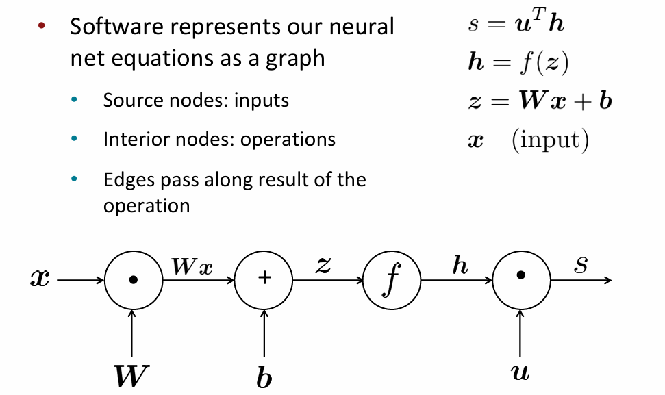
Backpropagation

按流程逐步计算各函数，从输入得到输出，即是正向传播(Forward Propagation)

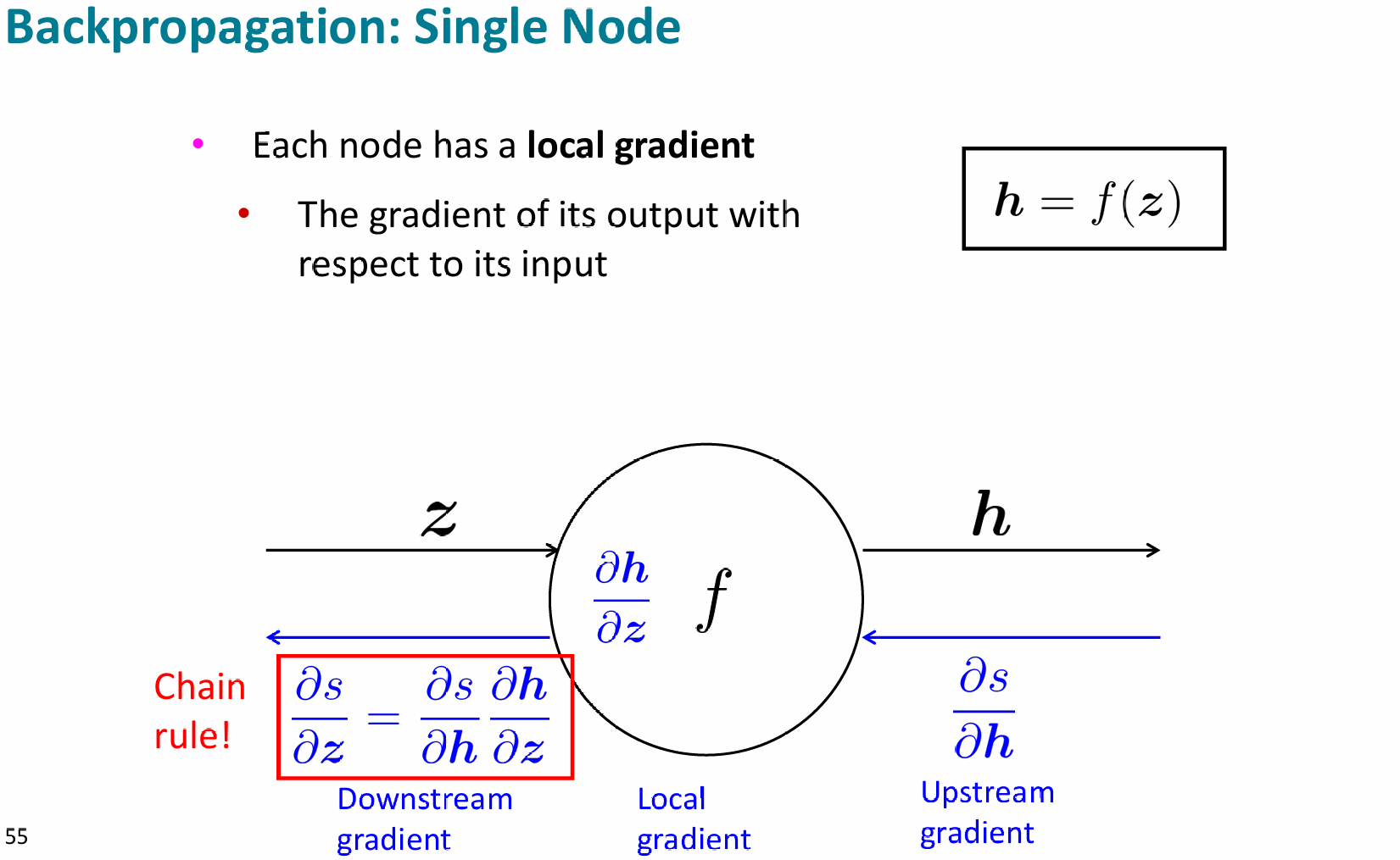
对于反向传播中的单个节点，有$downstream\ gradient=upstream\ gradient\times local\ gradient$

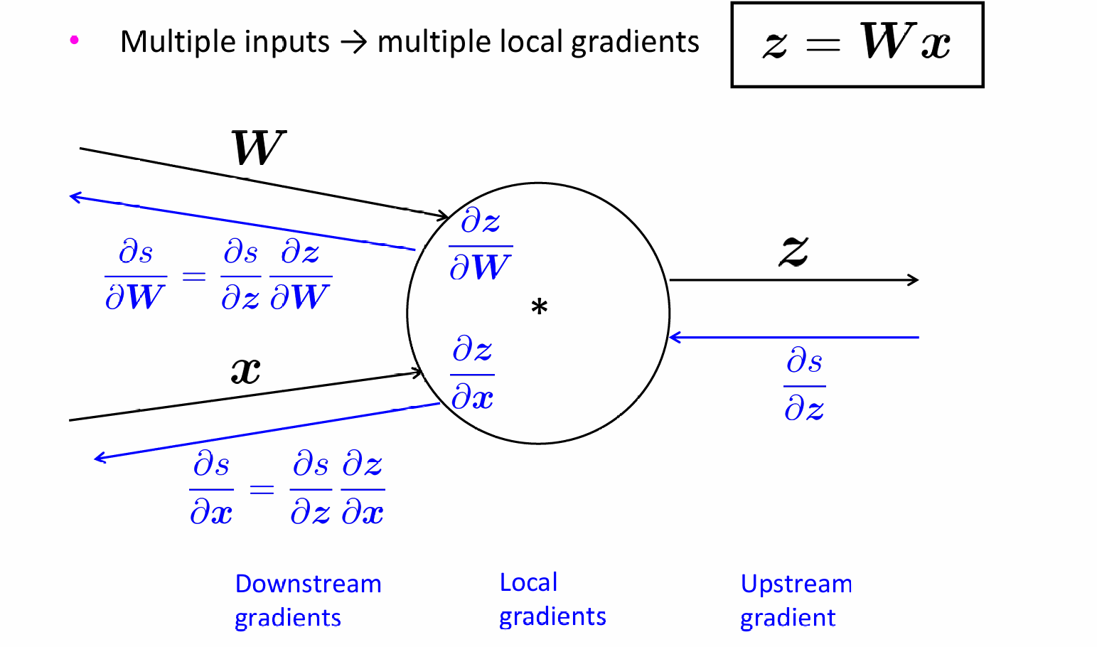
对于单节点的多输入，upstream gradient不变，各输入的local gradient不同，但计算公式是不变的

下面举个多输入的实际例子

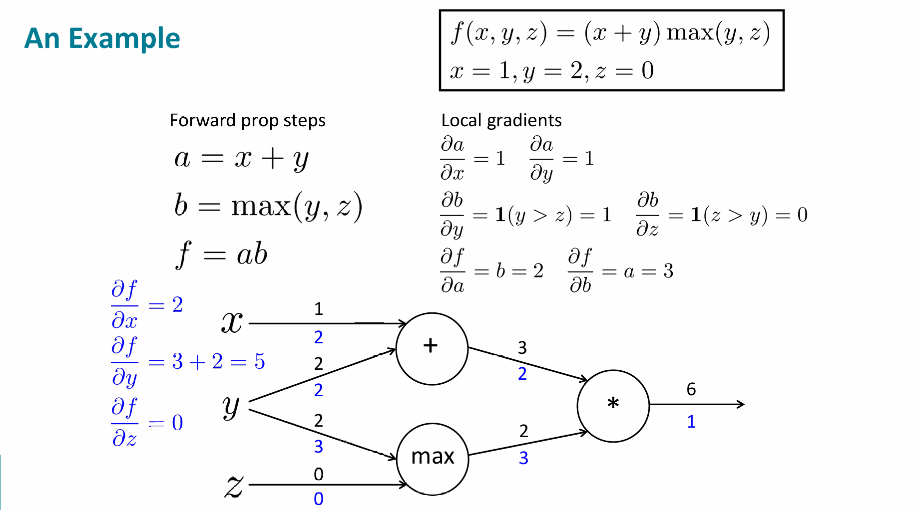
我们可以在这个基础上，假设输入y的值变为了2.1，那么$a=x+y=3.1$，$b=max(y+z)=y=2.1$，$a\times b=6.51$

所以，y值变化的0.1导致了结果0.51的变化，那么梯度就是$\frac{\Delta f}{\Delta y}=5.1$

Implementations

那么理论上，在已知正向传播的符号和计算的情况下，计算机可以自动得出反向传播的结果。但是在现代框架中，用户需手动设计局部导数的结算，这也比全自动方式提升了系统的运行效率和稳定性。

class MultiplyGate(object):
    def forward(self, x, y):
        z = x * y
        self.x = x  # must keep these around!
        self.y = y
        return z

    def backward(self, dz):
        dx = self.y * dz  # [dz/dx * dL/dz]
        dy = self.x * dz  # [dz/dy * dL/dz]
        return [dx, dy]

Numeric Gradient Checking

在手动推导和实现反向传播（Backprop）时，这是确保你数学公式没推错、代码没写错的标准验证方法：

$$f'(x) \approx \frac{f(x + h) - f(x - h)}{2h}$$

• 只需要前向传播函数 $f(x)$ 即可计算，不需要任何复杂的数学推导，不容易写错。
• 必须对模型的每一个参数分别进行两次前向传播（加 $h$ 和减 $h$），效率很低。
• 适合局部测试，不要对整个大型网络做验证，只针对某个特定层或小规模参数（如一个 $3 \times 3$ 的矩阵）进行。

Dependency Parsing

Syntactic Structure

• Phrase structure organizes words into nested constituents.

我们可以自己定义phrase构成的语法，比如名词短语可以是“限定词 + 形容词 + 名词”，“限定词 + 名词 + 介词短语”……介词短语可以是“介词 + 名词……”

• Dependency structure shows which words depend on (modify, attach to, or are arguments of) which other words

语言中很容易出现歧义(ambiguity)，在英语里有了介词短语，歧义就更多了，举个例子：

“Scientists count whales from space"可以理解为"Scientists [count] [whales from space]” 或者 “Scientists [count whales] [from space]” ……

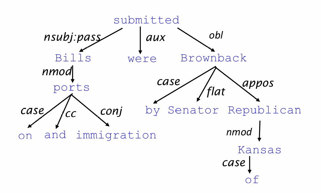
Dependency Grammar and Treebanks

Dependency syntax postulates that syntactic structure consists of relations between
lexical items, normally binary asymmetric relations (“arrows”) called dependencies

下图是个比较古老的"dependency structure"

An arrow connects a head (governor, superior, regent) with a dependent (modifier, inferior, subordinate)

Usually, dependencies form a tree (a connected, acyclic, single-root graph)

Annotated Data

起初，构建语言库（Treebank）似乎比手动编写语法规则要慢得多，且看起来没那么有用。手动标注数据确实是件麻烦的工作，但现在看来，却有很大的优势：

• 复用性(Reusability)：一套标注好的数据可以用来训练多种解析器（Parsers）、词性标注器（POS Taggers）
• 覆盖面广(Board coverage)：手动编写规则往往只能覆盖几个直觉上的例子，而标注真实语料可以涵盖语言在现实中的各种复杂用法。
• 频率与分布信息(Frequencies and distributional information)：它能告诉机器哪些结构更常见，帮助概率模型做出更准确的判断。
• 评估NLP(A way to evaluate NLP systems)：没有这套“标准”，我们就无法衡量一个 AI 模型的准确率（如 LAS/UAS 得分）

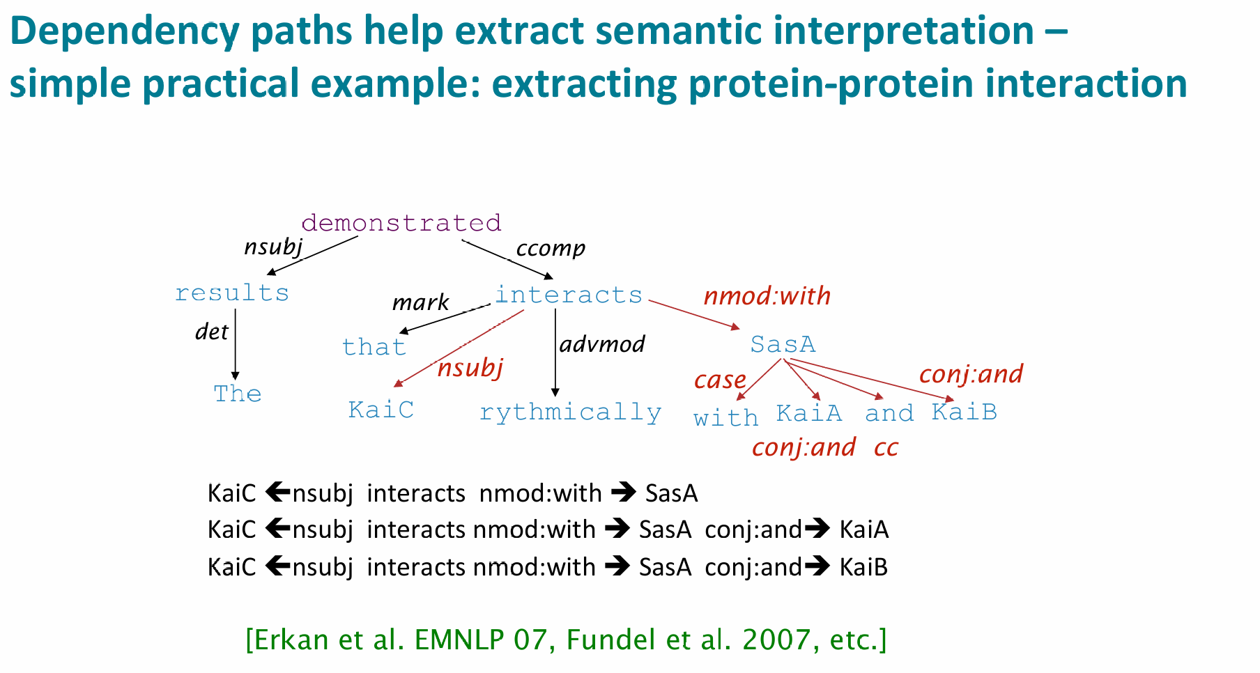
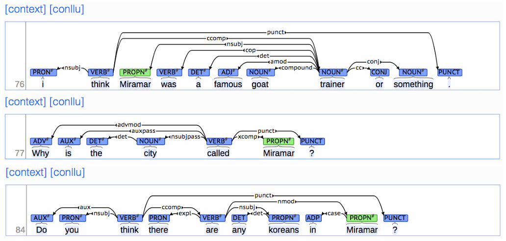
那么关于示例图中的各依存关系的意思，如下：

缩写	意思	简单理解
nsubj	名词主语	动作的发出者（如 I think）
nsubjpass	被动主语	被动语态里的主语（如 city called）
ccomp	从句	动词后面的整个小句子（如 think …）
advmod	状语修饰	修饰动词的程度、疑问等（如 Why）
amod	形容词修饰	修饰名词的形容词（如 famous goat）
compound	复合修饰	名词修饰名词（如 goat trainer）
det	限定关系	指向 a, the, any 等词
case	介词关系	指向 in, at 等介词
conj	并列关系	用 or, and 连接的词（如 trainer or something）

Dependency Conditioning Preferences

在进行句法分析时，计算机会根据“依存条件偏好（Dependency Conditioning Preferences）”来判断两个词之间是否存在依存关系：

• 双词亲和力 (Bilexical affinities)：依存关系（例如 [discussion → issues]）是合理的。
• 依存距离 (Dependency distance)：大多数（但并非所有）依存关系发生在邻近的单词之间。
• 介入材料 (Intervening material)：依存关系很少跨越中间的动词或标点符号。
• 中心词的价态 (Valency of heads)：对于一个中心词（Head）来说，通常在它的哪一侧会有多少个依存词？

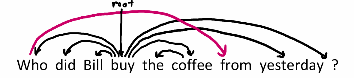
Projectivity

如果一个句子的单词按线性顺序排列，且所有的依存弧（dependency arcs）都画在单词上方时，没有任何两条弧线发生交叉，那么这个解析就是“投影的”。那么互出现了交叉，就是非投影的(non-projectivity)，说明发生了“长距离位移”或结构重叠。

但是现实中非投影的例子很常见，比如"Who did Bill buy the coffee from yesterday"

Transition-Based Dependency Parser

首先，这Transition-Based Dependency Parser分有一个Stack和一个Buffer，和三种操作：

Start: $ \sigma = [ROOT], \beta = w_1, …, w_n, A = \emptyset $

1. Shift: $\sigma, w_i | \beta, A \Rightarrow \sigma | w_i, \beta, A $

2. Left-$Arc_r$: $\sigma | w_i | w_j, \beta, A \Rightarrow \sigma | w_j, \beta, A \cup {r(w_j, w_i)} $

3. Right-$Arc_r$: $\sigma | w_i | w_j, \beta, A \Rightarrow \sigma | w_j, \beta, A \cup \{r(w_i, w_j)\}$

Finish: $\sigma = [w], \beta = \emptyset$

• σ（sigma）表示 堆栈（stack），存储当前正在处理或等待建立关系的词。

• β（beta）表示 缓冲区（buffer），存储尚未处理的输入词序列。

• A 表示 依存弧集合（set of dependency arcs），存储已建立的依存关系。

• Left-$Arc_r$ 和 Right-$Arc_r$ 是两种规约模型，用来表明一个词是另一个的依存词，以左或右方向。

那么下面先来举个例子：Analysis of “I ate fish”

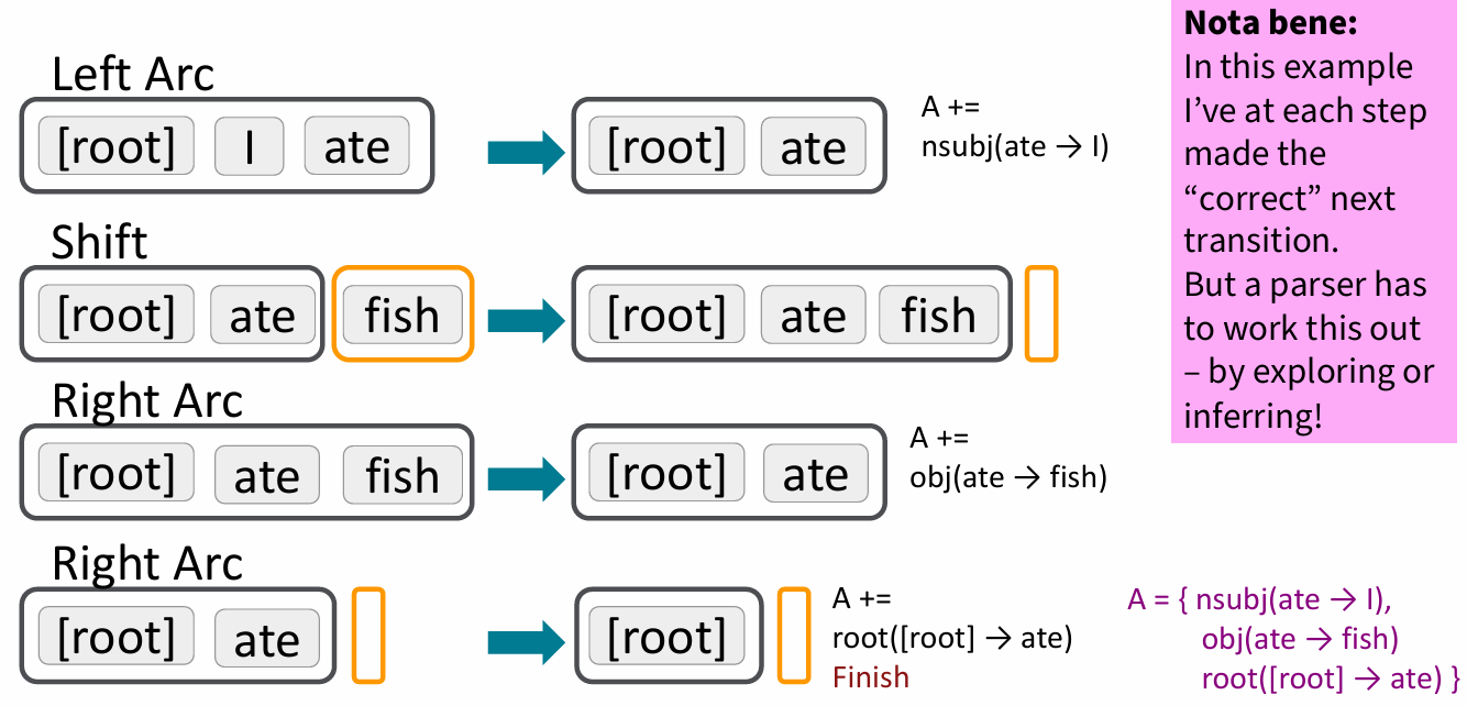
1. Left Arc操作 生成了一个由栈顶指向第二个元素的弧，建立了"ate"是中心词，"I"依存于"ate"的关系。然后将"I"移出栈。
2. Shift操作 将"fish"从缓冲区移入栈中
3. Right Arc操作 生成了一个由第二个元素指向栈顶元素的弧，建立了"ate"是中心词,"fish"依存于"ate"的关系。然后将"fish"移出栈。
4. 最后的Right Arc操作 使"[root]“指向"ate”，并在"ate"出栈后，只剩下根节点，操作完成。

Evaluation of Dependency Parsing

评价依存分析的指标分为UAS（无标签附件分数）和 LAS（有标签附件分数），下面是一个具体的例子: “[ROOT] She saw the video lecture.”，表中"Gold"是标准答案，"Parsed"是分析出的答案：

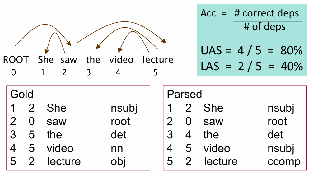
• 可见，UAS计算的是Head寻找得是否正确，本例中第三个"the"的依存词和标准不符。
• LAS计算的它们之间的关系类型是否标注正确，即Head和关系标签(label)都要一致，本例中只有"She"和"saw"是与标准相符的。

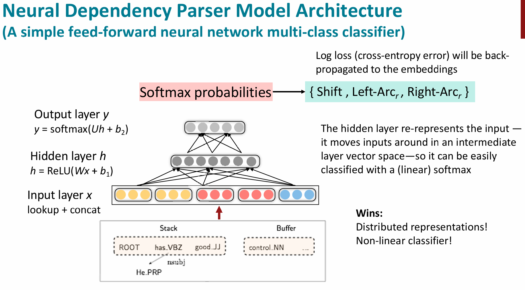
Neural dependency parsing

More than 95% of parsing time is consumed by feature computation

所以，我们可以用神经网络来加速特征提取，当然其方法还是基于上面的基于转移（Transition-based）的神经依存句法分析器。具体使用了了向量化、非线性等深度学习知识搭建出了第一个基于神经网络的依存分析器(2014年)。