Intro
These are my study notes for Stanford CS 224N: Natural Language Processing with Deep Learning, Spring 2024. The course covers word vectors, neural networks, dependency parsing, RNNs, LSTMs, Seq2Seq models, machine translation, attention, Transformers, and related NLP topics.
What is this course about?
Natural language processing is one of the most important technologies in the information age. Search, advertising, email, customer service, translation, virtual agents, medical reports, and many other systems all depend on language understanding. CS224N introduces both the foundations of deep learning for NLP and newer research around large language models, with assignments and projects implemented in PyTorch.
Word Vectors
$ vector("King") - vector("Man") + vector("Woman") $
This operation produces a vector close to the representation of Queen.
How do we have usable meaning in a computer?
The slides introduce several ways to represent meaning:
- WordNet
- one-hot vectors
- word vectors
The first two are useful, but they also have obvious limitations.
- WordNet relies on synonym sets and hypernym sets to define relationships between words. It is manually constructed, complex to maintain, and slow to absorb new words.
- One-hot vectors assign a symbol to every word. Even though the symbol is numeric, mathematically similar words are unrelated because their dot product is 0.
This leads to the famous distributional idea: You shall know a word by the company it keeps.
Word vectors normalize words into continuous vectors. Although a word may have multiple senses, its learned vector is often close to an average of its contextual usages. Dot products can then be used to measure relatedness between word vectors.
Word2vec
Word2vec captures the word-vector idea well: it compares a center word with nearby context words and learns a probability distribution from their similarity.
- We have a large corpus of text: a long list of words.
- Every word in a fixed vocabulary is represented by a vector.
- We go through each position $t$ in the text, where there is a center word $c$ and context, or outside, words $o$.
- We use the similarity between the vectors of $c$ and $o$ to calculate the probability of $o$ given $c$, or vice versa.
- We keep adjusting the word vectors to maximize this probability.

Objective Function
For each position $t=1,\ldots,T$, the model predicts context words within a fixed window of size $m$, given the center word $w_t$. The data likelihood is:
$$ L(\theta) = \prod_{t=1}^{T} \prod_{\substack{-m \le j \le m \\ j \neq 0}} P(w_{t+j} \mid w_t; \theta) $$For easier optimization and computation, this is converted into the average negative log likelihood:
$$ J(\theta) = -\frac{1}{T} \log L(\theta) = -\frac{1}{T} \sum_{t=1}^{T} \sum_{\substack{-m \le j \le m \\ j \neq 0}} \log P(w_{t+j} \mid w_t; \theta) $$Minimizing $J(\theta)$ is equivalent to maximizing prediction accuracy.
Prediction Function
$$ P(o \mid c) = \frac{\exp(u_o^T v_c)}{\sum_{w \in V} \exp(u_w^T v_c)} $$- $u_o^T v_c$: the larger the dot product, the closer the two words are in vector space, so the higher their semantic relatedness. Dot product compares the similarity of $o$ and $c$: $u^T v = u \cdot v = \sum_{i=1}^{n} u_i v_i$. A larger dot product means a larger probability.
- $\exp()$: maps any real number to a positive number. Because the exponential function grows quickly, it amplifies larger dot products and gives highly related words larger weights.
- $\sum_{w \in V} \exp(u_w^T v_c)$: the denominator sums over all possible words in vocabulary $V$. This ensures the probabilities over all possible outputs sum to 1.
This is an application of the softmax function:
$$ \text{softmax}(x_i) = \frac{\exp(x_i)}{\sum_{j=1}^{n} \exp(x_j)} = p_i $$- Softmax maps arbitrary values $x_i$ into a probability distribution $p_i$.
- “Max”: it amplifies the probability corresponding to the largest $x_i$.
- “Soft”: it still assigns some probability to smaller $x_i$ values.
To Train the Model
To train a model, we gradually adjust parameters to minimize a loss.
$$ \theta = \begin{bmatrix} v_{aardvark} \\ v_a \\ \vdots \\ v_{zebra} \\ u_{aardvark} \\ u_a \\ \vdots \\ u_{zebra} \end{bmatrix} \in \mathbb{R}^{2dV} $$- If the word-vector dimension is $d$ and the vocabulary size is $V$, the total number of parameters is $2dV$.
- Each word has two vectors. $\theta$ contains both representations for every word in the vocabulary: the center-word vector $v$ and the outside-word vector $u$.
- The model computes gradients for all parameters and updates them.
The gradient formula comes from differentiating the softmax loss. The math process is:
Initial loss function
For a center word $c$ and an outside word $o$, the negative log likelihood is:
$$ \text{Loss} = -\log P(o \mid c) $$Expand using the softmax definition
Substitute the formula for $P(o|c)$ and use log properties:
$$ \text{Loss} = -\log \left( \frac{\exp(u_o^T v_c)}{\sum_{w \in V} \exp(u_w^T v_c)} \right) = -u_o^T v_c + \log \sum_{w \in V} \exp(u_w^T v_c) $$Derivative of the first part
Differentiate the dot-product term with respect to the center-word vector $v_c$:
$$ \frac{\partial}{\partial v_c} (u_o^T v_c) = u_o $$Derivative of the second part
Apply the chain rule to the $\log \sum \exp(\dots)$ term:
$$ \frac{\partial}{\partial v_c} \log \sum_{w \in V} \exp(u_w^T v_c) = \frac{1}{\sum_{w \in V} \exp(u_w^T v_c)} \cdot \sum_{x \in V} \left[ \exp(u_x^T v_c) \cdot u_x \right] $$Rewrite it as an expectation under the probability distribution
Extract the original probability term $P(x|c)$:
$$ \sum_{x \in V} \left[ \frac{\exp(u_x^T v_c)}{\sum_{w \in V} \exp(u_w^T v_c)} \right] u_x = \sum_{x \in V} P(x \mid c) u_x $$Final gradient
Combining both parts gives the gradient used to update $v_c$:
$$ \frac{\partial \text{Loss}}{\partial v_c} = -u_o + \sum_{x \in V} P(x \mid c) u_x $$
Gradient Descent
Gradient descent update rule in matrix form:
$$ \theta^{new} = \theta^{old} - \alpha \nabla_{\theta} J(\theta) $$For a single parameter:
$$ \theta_j^{new} = \theta_j^{old} - \alpha \frac{\partial}{\partial \theta_j^{old}} J(\theta) $$- $\alpha$: step size or learning rate.
In practice, however, we usually use Stochastic Gradient Descent (SGD) instead.
- The objective function $J(\theta)$ is defined over all windows in the corpus. If every update required calculating the gradient $\nabla_{\theta} J(\theta)$ over the whole corpus, the computation would be extremely expensive.
- SGD does not compute the whole corpus each time. It repeatedly samples windows and updates parameters after each single window, or each small batch.
Skip-gram Model with Negative Sampling
$$ P(o\mid c)=\frac{\exp(u_x^T v_c)}{\sum_{w \in V} \exp(u_w^T v_c)} $$If we calculate probabilities with the traditional softmax, the denominator sums over all words, which is too expensive.
Skip-gram with Negative Sampling avoids calculating all possible words. Instead, it trains several logistic regression classifiers that prefer real context pairs over random context pairs. In practice, it samples $K$ negative examples, reducing the computation to $O(K)$:
$$ J_{neg-sample}(u_o, v_c, U) = -\log \sigma(u_o^T v_c) - \sum_{k \in \{K \text{ sampled indices}\}} \log \sigma(-u_k^T v_c) $$Here, $\sigma(x)=\frac{1}{1+e^{-x}}$ is the sigmoid function. It pushes positive pairs toward probability 1 and negative pairs toward probability 0.
However, this can make low-frequency words such as “zebra” too unlikely, while words like “the” are sampled too often. Therefore, the sampling distribution is adjusted with the $3/4$ power:
$$ P(W)=U(W)^{3/4}/Z $$This increases the relative probability of low-frequency words.
GloVe
Original GloVe paper: Global Vectors for Word Representation
Co-occurrence Matrix

Building a co-occurrence matrix is straightforward: first set a window size, then count the frequency of words that co-occur within that window. The figure above shows a simple example with window size 1, counting only neighboring words. However:
- The dimension of word vectors grows greatly as the vocabulary grows. This increases storage cost, makes the matrix very sparse, and makes models based on it less robust.
- Function words appear extremely often but provide little information.
- It does not reflect the relationship between word distance and word relatedness.
How can we reduce dimensionality? A classic method is SVD matrix factorization. I still do not fully understand the theory after asking AI, but in Assignment 1 a single sklearn function solves it.

- $X$ (co-occurrence matrix): size $|V| \times |V|$. Each element $X_{ij}$ represents how many times word $i$ and word $j$ co-occur in the corpus.
- $U$ and $V$ (orthogonal matrices): their column vectors are orthonormal. In NLP, each row of $U$ is often treated as the original embedding of a word.
- $\Sigma$ (diagonal matrix): the diagonal values $\sigma_1, \sigma_2, \dots$ are called singular values. They are sorted from large to small and represent the importance, variance, or information carried by each dimension.
Dimensionality reduction means compressing a word vector of length $V$ from the co-occurrence matrix into a vector of length $K$.
The key insight is that semantic meaning is not encoded by co-occurrence probabilities themselves, but by ratios of co-occurrence probabilities.
Ratios of co-occurrence probabilities can encode semantic components, and we want to capture these as linear semantic components in the word-vector space.
| $x = \text{solid}$ | $x = \text{gas}$ | $x = \text{water}$ | $x = \text{fashion}$ | |
|---|---|---|---|---|
| $P(x\mid\text{ice})$ | $1.9 \times 10^{-4}$ | $6.6 \times 10^{-5}$ | $3.0 \times 10^{-3}$ | $1.7 \times 10^{-5}$ |
| $P(x\mid\text{steam})$ | $2.2 \times 10^{-5}$ | $7.8 \times 10^{-4}$ | $2.2 \times 10^{-3}$ | $1.8 \times 10^{-5}$ |
| $\dfrac{P(x\mid\text{ice})}{P(x\mid\text{steam})}$ | $8.9$ | $8.5 \times 10^{-2}$ | $1.36$ | $0.96$ |
Analogies
Word vectors are mathematically powerful, but their analogy behavior has many practical problems.
In the following example, the question is $woman + grandfather - man = ?$. The obvious and most likely result is grandmother. But why do other words such as granddaughter and mother also receive almost equally high scores?
| |
| |
Although the assignment does not give a standard answer, this can be understood through semantic clustering.
- Semantic neighborhood effect
- In vector space, logically similar words often cluster together. When we calculate $\vec{w} + \vec{g} - \vec{m}$, we are actually locating a coordinate point in the space.
granddaughteralso has features such as “female” and “relative”, and often appears in contexts similar tograndfatherorgrandmother. Along the “family relation” dimension, these words are very close.
- Overlapping dimensions
- Word vectors usually have hundreds of dimensions. Although we subtract
manand addgrandfather, this does not completely erase similarity along other dimensions. daughter,mother, andgrandmothershare many dimensions such as[+female],[+human], and[+relative].
- Word vectors usually have hundreds of dimensions. Although we subtract
The next example is an incorrect analogy. The expected answer should be something like socks, but why does the model ignore glove and hand and output many square-related terms? Clearly this is not about foot as a body part, but about foot as a unit of length.
| |
| |
- Interference from polysemy
- As mentioned above,
footis also a unit of length, and it often combines withsquare.
- As mentioned above,
- Training corpus bias
- Since
foothas multiple meanings but the output is almost entirely about the unit sense, the training corpus may contain many...square footcontexts.
- Since
- Word choice
- Even though all outputs are
...squareterms, their scores are only around 0.5. This suggests the model did not find a strongly related word and probably did not understand the relationship amongglove,hand, andfoot.
- Even though all outputs are
Neural Network
A neural network = running several logistic regressions at the same time.
CS231n Deep Learning on Network Architectures
CS231n Deep Learning for Computer Vision on Backprop
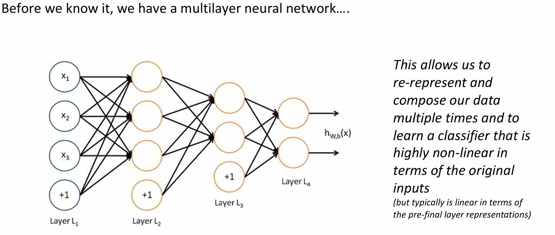
Structure

Non-linearities
Why do neural networks need non-linearities?
- Core idea: neural networks perform function approximation, such as regression or classification.
- Without non-linearity: a deep neural network can only perform linear transformations.
- More layers do not help: extra linear layers collapse into a single linear transformation: $W_1 W_2 x = Wx$.
- With non-linearity: a multi-layer structure with non-linear functions can approximate more complex functions.

- Bottom-left figures: the left figure shows linear classification, which can only draw a straight line and cannot separate complex red/green point distributions. The right figure shows non-linear classification, which can draw curves and separate the data.
- Three wave figures on the right: as function complexity increases, only non-linear models can fit the oscillating observed data.
The common non-linear activation functions were already covered in my Intelligent Computing Systems course, so I will not expand on them here.

Gradients
At a simple level, a gradient is a derivative with respect to a variable. For example:
$$ f(x)=x^3 $$Its derivative is:
$$ \frac{df}{dx}=3x^2 $$Of course, this is only a very simple example. In practice, neural networks involve large-scale chain rule calculations and gradients of matrices, or Jacobian matrices.
Chain Rule
In single-variable calculus, if $y = f(u)$ and $u = g(x)$, then:
$$ \frac{dy}{dx} = \frac{dy}{du} \cdot \frac{du}{dx} $$In neural networks, each layer is usually a vector, such as $\mathbf{h}, \mathbf{z} \in \mathbb{R}^n$. When this logic is extended to vectors, multiplication becomes matrix multiplication.
For multiple variables, we multiply Jacobian matrices:
Suppose $\mathbf h= f(z)$ and $\mathbf z=Wx+b$. The partial derivatives below form Jacobian matrices:
$$ \frac{\partial \mathbf{h}}{\partial \mathbf{x}} = \frac{\partial \mathbf{h}}{\partial \mathbf{z}} \frac{\partial \mathbf{z}}{\partial \mathbf{x}} $$Matrix Calculus
From the following expression, the Jacobian has non-zero values only on the diagonal:
$$ \begin{aligned} \left( \frac{\partial \mathbf{h}}{\partial \mathbf{z}} \right)_{ij} &= \frac{\partial h_i}{\partial z_j} = \frac{\partial}{\partial z_j} f(z_i) \quad && \text{definition of Jacobian} \\ &= \begin{cases} f'(z_i) & \text{if } i = j \\ 0 & \text{if otherwise} \end{cases} \quad && \text{regular 1-variable derivative} \end{aligned} $$$$ \frac{\partial \mathbf h}{\partial \mathbf z} = \begin{pmatrix} f'(z_1) & 0 & \cdots & 0 \\ 0 & f'(z_2) & \cdots & 0 \\ \vdots & \vdots & \ddots & \vdots \\ 0 & 0 & \cdots & f'(z_n) \end{pmatrix} = \operatorname{diag}(f'(\mathbf z)) $$Another common Jacobian is:
$$ \frac{\partial}{\partial \mathbf{u}}(\mathbf{u}^T \mathbf{h})=\mathbf h^T $$Suppose $\mathbf{u}$ and $\mathbf{h}$ are both $n$-dimensional column vectors:
$$ \mathbf{u} = \begin{bmatrix} u_1 \\ u_2 \\ \vdots \\ u_n \end{bmatrix}, \quad \mathbf{h} = \begin{bmatrix} h_1 \\ h_2 \\ \vdots \\ h_n \end{bmatrix} $$Their inner product is a scalar:
$$ f = \mathbf{u}^T \mathbf{h} = u_1 h_1 + u_2 h_2 + \dots + u_n h_n = \sum_{i=1}^n u_i h_i $$We want to differentiate with respect to vector $\mathbf{u}$. According to the definition of a Jacobian, we differentiate with respect to each element $u_k$:
$$ \frac{\partial f}{\partial u_k} = \frac{\partial}{\partial u_k} (u_1 h_1 + \dots + u_k h_k + \dots + u_n h_n) $$All terms except $u_k h_k$ do not contain $u_k$, so their derivatives are 0:
$$ \frac{\partial f}{\partial u_k} = h_k $$By the usual Jacobian convention, the derivative of a scalar with respect to a column vector is a row vector:
$$ \frac{\partial f}{\partial \mathbf{u}} = \begin{bmatrix} \frac{\partial f}{\partial u_1} & \frac{\partial f}{\partial u_2} & \dots & \frac{\partial f}{\partial u_n} \end{bmatrix} = \begin{bmatrix} h_1 & h_2 & \dots & h_n \end{bmatrix} = \mathbf{h}^T $$Write out the Jacobians
$$ \begin{aligned} \frac{\partial s}{\partial \mathbf{b}} &= \frac{\partial s}{\partial \mathbf{h}} \frac{\partial \mathbf{h}}{\partial \mathbf{z}} \frac{\partial \mathbf{z}}{\partial \mathbf{b}} \\ &= \mathbf{u}^T \text{diag}(f'(\mathbf{z})) \mathbf{I} \\ &= \mathbf{u}^T \odot f'(\mathbf{z}) \end{aligned} $$$\odot$ = Hadamard product = element-wise multiplication of two vectors to produce a vector.
| Variable | Meaning in neural networks | Note |
|---|---|---|
| $s$ | Loss/score | The final scalar output, such as cross-entropy loss. We want to know how it changes with parameters. |
| $\mathbf{b}$ | Bias vector | A learnable parameter in the current layer. |
| $\mathbf{z}$ | Logits/pre-activation | The result of the linear combination: $\mathbf{z} = \mathbf{W}\mathbf{x} + \mathbf{b}$. |
| $\mathbf{h}$ | Activation/hidden state | The output after applying a non-linear activation: $\mathbf{h} = f(\mathbf{z})$. |
| $\mathbf{u}^T$ | Upstream gradient $\frac{\partial s}{\partial \mathbf{h}}$ | The signal propagated backward from higher layers. |
| $f'(\mathbf{z})$ | Derivative of the activation function | For example, the derivative of ReLU or sigmoid. It determines which neurons are active. |
| $\mathbf{I}$ | Identity matrix | Since $\mathbf{z} = \dots + \mathbf{b}$, the derivative of $\mathbf{z}$ with respect to $\mathbf{b}$ is 1, represented as the identity matrix. |
Re-using Computation
The upstream error signal $\boldsymbol{\delta}$ is:
$$ \boldsymbol{\delta} = \frac{\partial s}{\partial \mathbf{h}} \frac{\partial \mathbf{h}}{\partial \mathbf{z}} = \mathbf{u}^T \circ f'(\mathbf{z}) $$After computing $\boldsymbol{\delta}$ first, later calculations become simpler:
Gradient of the weight matrix $W$:
$$ \frac{\partial s}{\partial \mathbf{W}} = \boldsymbol{\delta} \frac{\partial \mathbf{z}}{\partial \mathbf{W}} $$Gradient of the bias vector $\mathbf{b}$:
$$ \frac{\partial s}{\partial \mathbf{b}} = \boldsymbol{\delta} \frac{\partial \mathbf{z}}{\partial \mathbf{b}} = \boldsymbol{\delta} $$
Shape Convention
Suppose the weight matrix is $\mathbf{W} \in \mathbb{R}^{n \times m}$ and the output is a scalar $s$, such as a loss. By the pure mathematical definition, $\frac{\partial s}{\partial \mathbf{W}}$ should be a $1 \times nm$ row vector, a Jacobian. But if we use this form directly, the gradient update rule $\theta^{new} = \theta^{old} - \alpha \nabla_{\theta} J(\theta)$ cannot subtract tensors because the shapes do not match.
For convenience in computation, we use the convention that the gradient shape should match the parameter shape. Therefore, $\frac{\partial s}{\partial \mathbf{W}}$ is also an $n \times m$ matrix:
$$ \frac{\partial s}{\partial \mathbf{W}} = \begin{bmatrix} \frac{\partial s}{\partial W_{11}} & \dots & \frac{\partial s}{\partial W_{1m}} \\ \vdots & \ddots & \vdots \\ \frac{\partial s}{\partial W_{n1}} & \dots & \frac{\partial s}{\partial W_{nm}} \end{bmatrix} $$$$ \frac{\partial s}{\partial \mathbf{W}} = \boldsymbol{\delta}^T \mathbf{x}^T $$So what shape should a derivative result take?
The practical answer is to follow the shape convention:
- Method: do not get stuck on the strict Jacobian definition. Always watch the variable dimensions.
- Core trick: use dimensional analysis to decide when to transpose a term or adjust multiplication order, so each layer’s gradient has exactly the same shape as the corresponding parameter.
- Important conclusion about $\boldsymbol{\delta}$: the error signal propagated to a hidden layer should have the same dimension as the number of neurons in that hidden layer, or the dimension of its activation vector.
Backpropagation
Computing each function step by step from input to output is forward propagation.

For a single node in backpropagation:
$$ downstream\ gradient = upstream\ gradient \times local\ gradient $$
For a node with multiple inputs, the upstream gradient remains the same, but each input has a different local gradient. The formula is unchanged.

Here is a concrete example with multiple inputs:

Based on this example, suppose the input value $y$ changes to 2.1. Then $a=x+y=3.1$, $b=max(y+z)=y=2.1$, and $a\times b=6.51$.
So a change of 0.1 in $y$ causes a change of 0.51 in the result. The gradient is:
$$ \frac{\Delta f}{\Delta y}=5.1 $$Implementations
In theory, once the symbolic computation of forward propagation is known, a computer can automatically derive the result of backpropagation. But in modern frameworks, users or framework authors still define local derivative rules. This is more efficient and stable than a fully automatic symbolic approach.
| |
Numeric Gradient Checking
When manually deriving and implementing backpropagation, numeric gradient checking is the standard way to verify that the math and code are correct:
$$ f'(x) \approx \frac{f(x + h) - f(x - h)}{2h} $$- It only needs the forward function $f(x)$, so it does not require complex mathematical derivation and is less likely to be wrong.
- It must run two forward passes for each parameter, one with $+h$ and one with $-h$, so it is inefficient.
- It is suitable for local tests, not for validating a large whole network. Use it for a specific layer or a small parameter tensor, such as a $3 \times 3$ matrix.
Dependency Parsing
Syntactic Structure
- Phrase structure organizes words into nested constituents.
We can define grammar rules for phrases ourselves. For example, a noun phrase can be “determiner + adjective + noun” or “determiner + noun + prepositional phrase”; a prepositional phrase can be “preposition + noun”, and so on.
- Dependency structure shows which words depend on, modify, attach to, or act as arguments of other words.
Ambiguity is common in language, and prepositional phrases create even more ambiguity in English. For example:
Scientists count whales from space
This can be understood as Scientists [count] [whales from space], or Scientists [count whales] [from space].

Dependency Grammar and Treebanks
Dependency syntax assumes that syntactic structure consists of relations between lexical items, usually binary asymmetric relations called dependencies.
The figure below is an older example of a dependency structure.
An arrow connects a head, also called governor, superior, or regent, with a dependent, also called modifier, inferior, or subordinate.
Usually, dependencies form a tree: a connected, acyclic, single-root graph.

Annotated Data

At first, building a treebank may look slower than manually writing grammar rules, and perhaps less useful. Manual annotation is indeed troublesome, but it has several major advantages:
- Reusability: one annotated dataset can be used to train many parsers and POS taggers.
- Broad coverage: hand-written rules often cover only a few intuitive examples, while annotated real corpora cover the complexity of language in actual use.
- Frequencies and distributional information: a treebank tells the model which structures are more common, helping probabilistic models make better decisions.
- A way to evaluate NLP systems: without this kind of gold standard, we cannot measure parser accuracy through metrics such as LAS and UAS.
The dependency labels in the example figure can be roughly understood as:
| Label | Meaning | Simple understanding |
|---|---|---|
| nsubj | Nominal subject | The doer of the action, as in I think. |
| nsubjpass | Passive subject | The subject in passive voice, as in city called. |
| ccomp | Clausal complement | A clause after a verb, as in think …. |
| advmod | Adverbial modifier | Modifies degree, question words, or verbs, as in Why. |
| amod | Adjectival modifier | An adjective modifying a noun, as in famous goat. |
| compound | Compound modifier | A noun modifying another noun, as in goat trainer. |
| det | Determiner | Points to words like a, the, any. |
| case | Case marker | Points to prepositions such as in, at. |
| conj | Conjunction | Words connected by or, and, as in trainer or something. |
Dependency Conditioning Preferences
During parsing, the model uses dependency conditioning preferences to judge whether two words are likely to have a dependency relation:
- Bilexical affinities: whether a dependency such as
[discussion -> issues]is reasonable. - Dependency distance: most, but not all, dependencies occur between nearby words.
- Intervening material: dependencies rarely cross intervening verbs or punctuation.
- Valency of heads: for a head word, how many dependents does it usually have on each side?
Projectivity
If the words of a sentence are arranged in linear order and all dependency arcs are drawn above the words, a parse is projective when no two arcs cross. If arcs cross, the parse is non-projective, which usually indicates long-distance movement or overlapping structure.
Non-projective examples are common in real language, such as:
Who did Bill buy the coffee from yesterday

Transition-Based Dependency Parser
A transition-based dependency parser has a stack, a buffer, and three operations.
Start: $\sigma = [ROOT], \beta = w_1, ..., w_n, A = \emptyset$
Shift: $\sigma, w_i | \beta, A \Rightarrow \sigma | w_i, \beta, A $
Left-$Arc_r$: $\sigma | w_i | w_j, \beta, A \Rightarrow \sigma | w_j, \beta, A \cup \{r(w_j, w_i)\} $
Right-$Arc_r$: $\sigma | w_i | w_j, \beta, A \Rightarrow \sigma | w_j, \beta, A \cup \{r(w_i, w_j)\}$
Finish: $\sigma = [w], \beta = \emptyset$
- $\sigma$ represents the stack, storing words currently being processed or waiting for dependency relations.
- $\beta$ represents the buffer, storing the input words that have not yet been processed.
- $A$ represents the set of dependency arcs, storing dependency relations already created.
- Left-$Arc_r$ and Right-$Arc_r$ are two reduction operations that establish whether one word depends on another, with left or right direction.
Now consider the example: analysis of I ate fish.
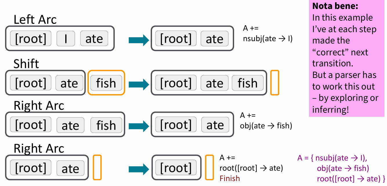
- The Left Arc operation creates an arc from the stack top toward the second element, establishing that
ateis the head andIdepends onate. ThenIis removed from the stack. - The Shift operation moves
fishfrom the buffer into the stack. - The Right Arc operation creates an arc from the second element to the stack top, establishing that
ateis the head andfishdepends onate. Thenfishis removed from the stack. - The final Right Arc operation makes
[root]point toate. Afterateis popped, only the root node remains and parsing is complete.
Evaluation of Dependency Parsing
Dependency parsing is evaluated with UAS (Unlabeled Attachment Score) and LAS (Labeled Attachment Score). The following example uses [ROOT] She saw the video lecture.; Gold is the standard answer and Parsed is the parser output.

- UAS checks whether the
Headis correct. In this example, the third wordthehas a different head from the gold parse. - LAS checks whether both the
Headand the relation label are correct. In this example, only the relation betweenSheandsawmatches the gold parse.
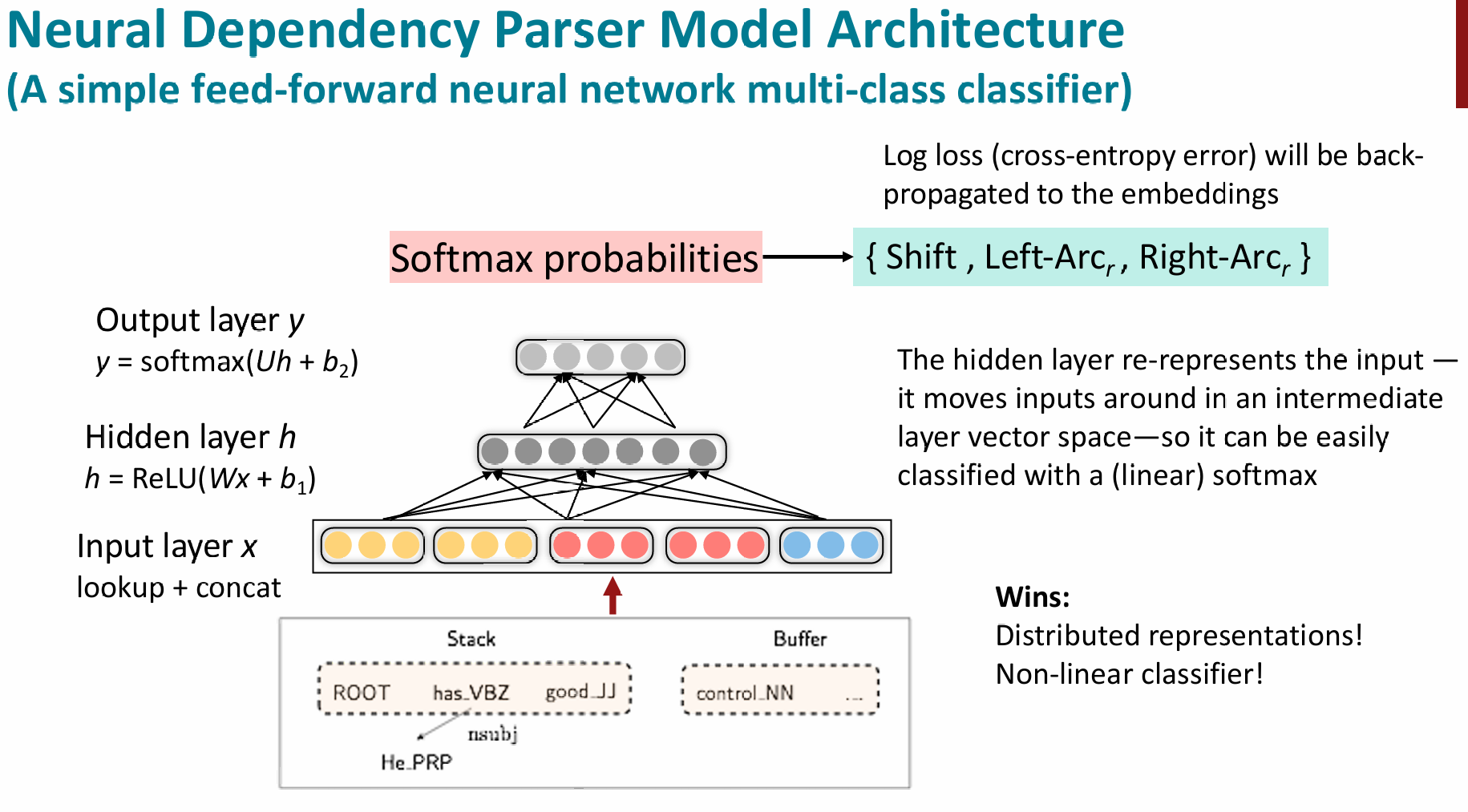
Neural dependency parsing
More than 95% of parsing time is consumed by feature computation.
Therefore, neural networks can be used to accelerate feature extraction. The method is still based on the transition-based dependency parser above, but it uses vectorization and non-linear neural network modeling. This led to the first neural-network-based dependency parser in 2014.
Recurrent Neural Networks
Language Modeling
In simple terms, a language model takes text, or tokens, as input and outputs probabilities.
$$ \begin{aligned} P(\boldsymbol{x}^{(1)}, \dots, \boldsymbol{x}^{(T)}) &= P(\boldsymbol{x}^{(1)}) \times P(\boldsymbol{x}^{(2)} | \boldsymbol{x}^{(1)}) \times \dots \times P(\boldsymbol{x}^{(T)} | \boldsymbol{x}^{(T-1)}, \dots, \boldsymbol{x}^{(1)}) \\ &= \prod_{t=1}^{T} \underbrace{P(\boldsymbol{x}^{(t)} | \boldsymbol{x}^{(t-1)}, \dots, \boldsymbol{x}^{(1)})}_{\text{This is what our LM provides}} \end{aligned} $$$P(\boldsymbol{x}^{(1)}, \dots, \boldsymbol{x}^{(T)})$ is the probability of an entire sequence, such as a sentence. By decomposing the joint probability into a product of conditional probabilities using the chain rule, we can calculate the probability of the sequence. The core task of a language model is to use the previous context $\boldsymbol{x}^{(t-1)}, \dots, \boldsymbol{x}^{(1)}$ to predict the probability of the next token $\boldsymbol{x}^{(t)}$.
n-gram Language Models
An n-gram is a chunk of $n$ consecutive words. Here, $n$ means how many words form one unit. To build an n-gram language model:
First, make a Markov assumption: the word $x^{(t+1)}$ depends only on the previous $n-1$ words.
$$ P(x^{(t+1)} | x^{(t)}, \dots, x^{(1)}) = P(x^{(t+1)} | \underbrace{x^{(t)}, \dots, x^{(t-n+2)}}_{n-1 \text{ words}}) \quad \text{(assumption)} $$Using the definition of conditional probability, the above formula can be written as the ratio between an n-gram probability and an $(n-1)$-gram probability:
$$ = \frac{P(x^{(t+1)}, x^{(t)}, \dots, x^{(t-n+2)}) \leftarrow \text{prob of a n-gram}}{P(x^{(t)}, \dots, x^{(t-n+2)}) \leftarrow \text{prob of a (n-1)-gram}} \quad \text{(definition of conditional prob)} $$We approximate these probabilities by counting n-gram frequencies in a large text corpus:
$$ \approx \frac{\text{count}(x^{(t+1)}, x^{(t)}, \dots, x^{(t-n+2)})}{\text{count}(x^{(t)}, \dots, x^{(t-n+2)})} \quad \text{(statistical approximation)} $$
For example, suppose we have a 4-gram language model and want to predict the last blank:
as the proctor started the clock, the students opened their ......
We only use the last three words, students opened their:
According to the corpus, students opened their books may appear most often, while the more contextually appropriate students opened their exams may appear less often.
Problems with n-gram Language Models
When using counting to estimate probabilities, we face sparsity problems:
If the phrase
students opened their $w$never appears in the training data, then the probability for any such $w$ becomes 0.This can be handled by adding a small value $\delta$ to the count of each word $w \in V$, which is smoothing.
If the prefix
students opened theirnever appears in the training data, then we cannot calculate the probability of any $w$ because the denominator is 0.In this case, we back off to a shorter context, such as
opened their.
There is also a storage problem:
- We need to store counts for all observed n-grams in the corpus.
- If $n$ increases, the required corpus size and storage grow greatly.
A Fixed-window Neural Language Model

Input layer (words / one-hot vectors): the inputs are one-hot vectors of words $\boldsymbol{x}^{(1)}, \boldsymbol{x}^{(2)}, \boldsymbol{x}^{(3)}, \boldsymbol{x}^{(4)}$.
Embedding layer (concatenated word embeddings): words are converted into dense embeddings and concatenated:
$$ \boldsymbol{e} = [\boldsymbol{e}^{(1)}; \boldsymbol{e}^{(2)}; \boldsymbol{e}^{(3)}; \boldsymbol{e}^{(4)}] $$Hidden layer: apply a linear transformation with weight matrix $W$ and bias $b_1$, then pass through an activation function $f$, usually tanh or ReLU:
$$ \boldsymbol{h} = f(W\boldsymbol{e} + \boldsymbol{b}_1) $$Output distribution: apply weight matrix $U$ and bias $b_2$, then use softmax to produce a probability distribution over vocabulary $V$:
$$ \hat{\boldsymbol{y}} = \text{softmax}(U\boldsymbol{h} + \boldsymbol{b}_2) \in \mathbb{R}^{|V|} $$
Compared with n-gram methods, this improves:
- Sparsity problem: it no longer relies on exact counts, and can generalize unseen word groups through vector-space similarity.
- Storage: it does not need to store frequencies for all observed n-grams, only model parameters.
But some problems remain:
- Fixed-window limitation
- The fixed context window is usually too small.
- Increasing the window size linearly increases the number of parameters in weight matrix $W$.
- No matter how large the window is, it cannot capture long-range dependencies outside the window.
- Lack of symmetry
- Inputs $\boldsymbol{x}^{(1)}$ and $\boldsymbol{x}^{(2)}$ are multiplied by completely different parts of $W$, so the model does not process each input position consistently.
RNN Language Model
The Unreasonable Effectiveness of Recurrent Neural Networks

Advantages of RNNs:
- They can process input of any length.
- In theory, computation at step $t$ can use information from many steps earlier.
- Fixed model size: increasing input length does not increase the number of model parameters.
- Symmetry: the same weights are applied at every step, so input positions are processed consistently.
Disadvantages of RNNs:
- Slow computation: because computation is recurrent, it cannot be fully parallelized.
- Practical difficulty: in practice, it is hard to use information from many steps earlier, because of vanishing or exploding gradients.
Train an RNN Language Model
Obtain a large text corpus consisting of a word sequence $\boldsymbol{x}^{(1)}, \dots, \boldsymbol{x}^{(T)}$.
Feed the sequence into the RNN-LM and compute the output distribution $\hat{\boldsymbol{y}}^{(t)}$ for every time step $t$. This means the model predicts the probability distribution over possible next words at each position, given the words seen so far.
The model produces a loss at every time step. At step $t$, the loss is the cross entropy between the predicted distribution $\hat{\boldsymbol{y}}^{(t)}$ and the true next word $\boldsymbol{y}^{(t)}$, which is the one-hot vector of $\boldsymbol{x}^{(t+1)}$:
$$ J^{(t)}(\theta) = CE(\boldsymbol{y}^{(t)}, \hat{\boldsymbol{y}}^{(t)}) = - \sum_{w \in V} \boldsymbol{y}^{(t)}_w \log \hat{\boldsymbol{y}}^{(t)}_w = - \log \hat{\boldsymbol{y}}^{(t)}_{\boldsymbol{x}_{t+1}} $$To get the loss over the whole training sequence, average the loss over all steps:
$$ J(\theta) = \frac{1}{T} \sum_{t=1}^{T} J^{(t)}(\theta) = \frac{1}{T} \sum_{t=1}^{T} - \log \hat{\boldsymbol{y}}^{(t)}_{\boldsymbol{x}_{t+1}} $$This uses the idea of teacher forcing: when calculating loss, the model does not feed its own previous prediction into the next step. It directly uses the correct word from the corpus.
Computing the loss and gradients over the entire corpus $\boldsymbol{x}^{(1)}, \dots, \boldsymbol{x}^{(T)}$ at once is extremely expensive in memory. In practice, we treat the sequence as sentences or documents, use SGD to compute loss and gradients over a small chunk of data, and update parameters immediately.
Backpropagation for RNN
RNN parameters are trained with backpropagation through time. The backward pass runs along time steps $i=t,\dots,0$ and accumulates gradients.
Because $\boldsymbol{W}_h$ is shared at every time step, the total gradient is the sum of gradients produced at each step:
$$ \frac{\partial J^{(t)}}{\partial \boldsymbol{W}_h} = \sum_{i=1}^{t} \left. \frac{\partial J^{(t)}}{\partial \boldsymbol{W}_h} \right|_{(i)} \frac{\partial \boldsymbol{W}_h|_{(i)}}{\partial \boldsymbol{W}_h} = \sum_{i=1}^{t} \left. \frac{\partial J^{(t)}}{\partial \boldsymbol{W}_h} \right|_{(i)} $$As the sequence grows longer, full backpropagation becomes very expensive and is prone to vanishing or exploding gradients. In practice, training is often truncated after about 20 time steps.
Exploding Gradient
Exploding gradients occur when:
- The eigenvalues of $W_h$, roughly the magnitude of the weights, are greater than 1.
- As time step $T$ increases, gradients grow exponentially.
- Model weights are updated too aggressively, making the network unstable. Parameters may overflow into NaN and training collapses.
If the norm of the gradient exceeds a preset threshold before updating model parameters, we scale it down proportionally. If $\|\hat{\boldsymbol{g}}\| \ge threshold$, we apply gradient clipping:
$$ \hat{\boldsymbol{g}} \leftarrow \frac{threshold}{\|\hat{\boldsymbol{g}}\|} \hat{\boldsymbol{g}} $$Gradient clipping keeps the update in the same direction, but takes a smaller step.
Vanishing Gradient
Vanishing gradients occur when:
- The eigenvalues of $W_h$ are less than 1, or the derivatives of activation functions such as $f$ or tanh are less than 1.
- Gradients shrink exponentially as the number of backward steps increases.
- This corresponds to the RNN limitation mentioned earlier: in practice, it is hard to access information from many steps earlier. When gradients become extremely small, far-away weights are barely updated, and the model “forgets” long-term context.
For a vanilla RNN, learning to preserve information across many time steps is difficult because the hidden state $\boldsymbol{h}^{(t)}$ is constantly rewritten:
$$ \boldsymbol{h}^{(t)} = \sigma(\boldsymbol{W}_h \boldsymbol{h}^{(t-1)} + \boldsymbol{W}_x \boldsymbol{x}^{(t)} + \boldsymbol{b}) $$Therefore, we introduce independent memory, such as LSTMs, or build more direct connections, such as attention mechanisms.
Long Short-Term Memory
Understanding LSTM Networks – colah’s blog
Forget gate: controls what to keep and what to forget from the previous cell state.
$$ \boldsymbol{f}^{(t)} = \sigma (\boldsymbol{W}_f \boldsymbol{h}^{(t-1)} + \boldsymbol{U}_f \boldsymbol{x}^{(t)} + \boldsymbol{b}_f) $$Input gate: controls which parts of the new cell content are written into the cell.
$$ \boldsymbol{i}^{(t)} = \sigma (\boldsymbol{W}_i \boldsymbol{h}^{(t-1)} + \boldsymbol{U}_i \boldsymbol{x}^{(t)} + \boldsymbol{b}_i) $$Output gate: controls which parts of the cell are output to the hidden state.
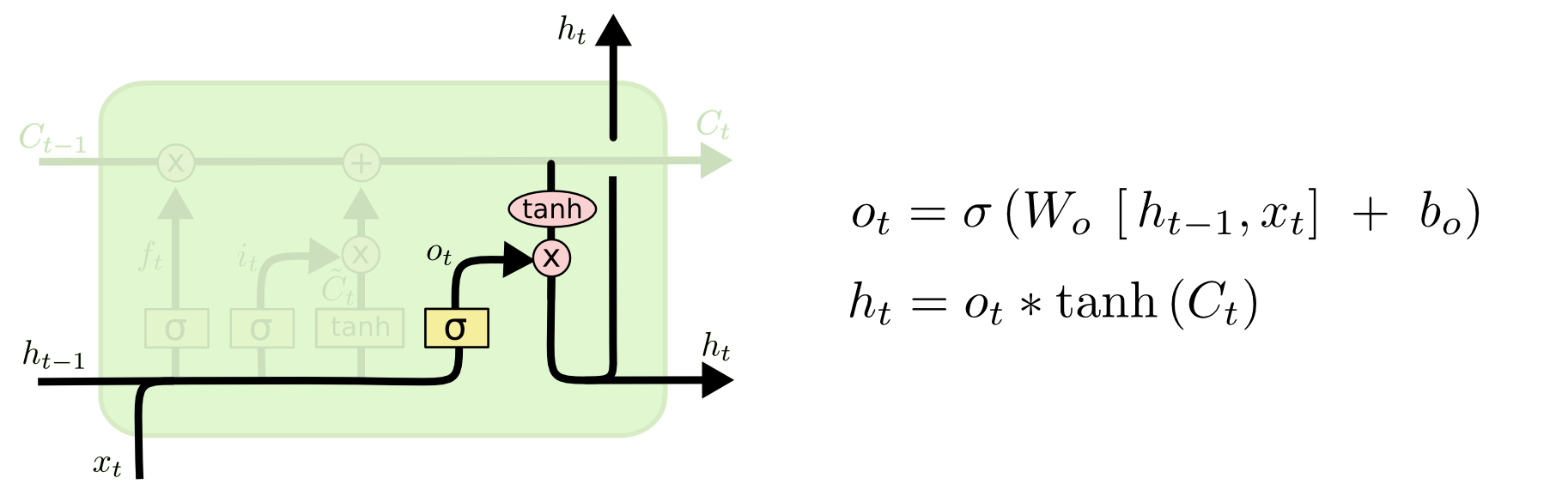
$$ \boldsymbol{o}^{(t)} = \sigma (\boldsymbol{W}_o \boldsymbol{h}^{(t-1)} + \boldsymbol{U}_o \boldsymbol{x}^{(t)} + \boldsymbol{b}_o) $$New cell content: the new content to be written into the cell, also known as candidate content.
$$ \tilde{\boldsymbol{c}}^{(t)} = \tanh (\boldsymbol{W}_c \boldsymbol{h}^{(t-1)} + \boldsymbol{U}_c \boldsymbol{x}^{(t)} + \boldsymbol{b}_c) $$Cell state: erase, or forget, parts of the previous cell state and write in new cell content.
$$ \boldsymbol{c}^{(t)} = \boldsymbol{f}^{(t)} \odot \boldsymbol{c}^{(t-1)} + \boldsymbol{i}^{(t)} \odot \tilde{\boldsymbol{c}}^{(t)} $$Hidden state: read, or output, some content from the cell.
$$ \boldsymbol{h}^{(t)} = \boldsymbol{o}^{(t)} \odot \tanh \boldsymbol{c}^{(t)} $$Step-by-Step LSTM Walk Through
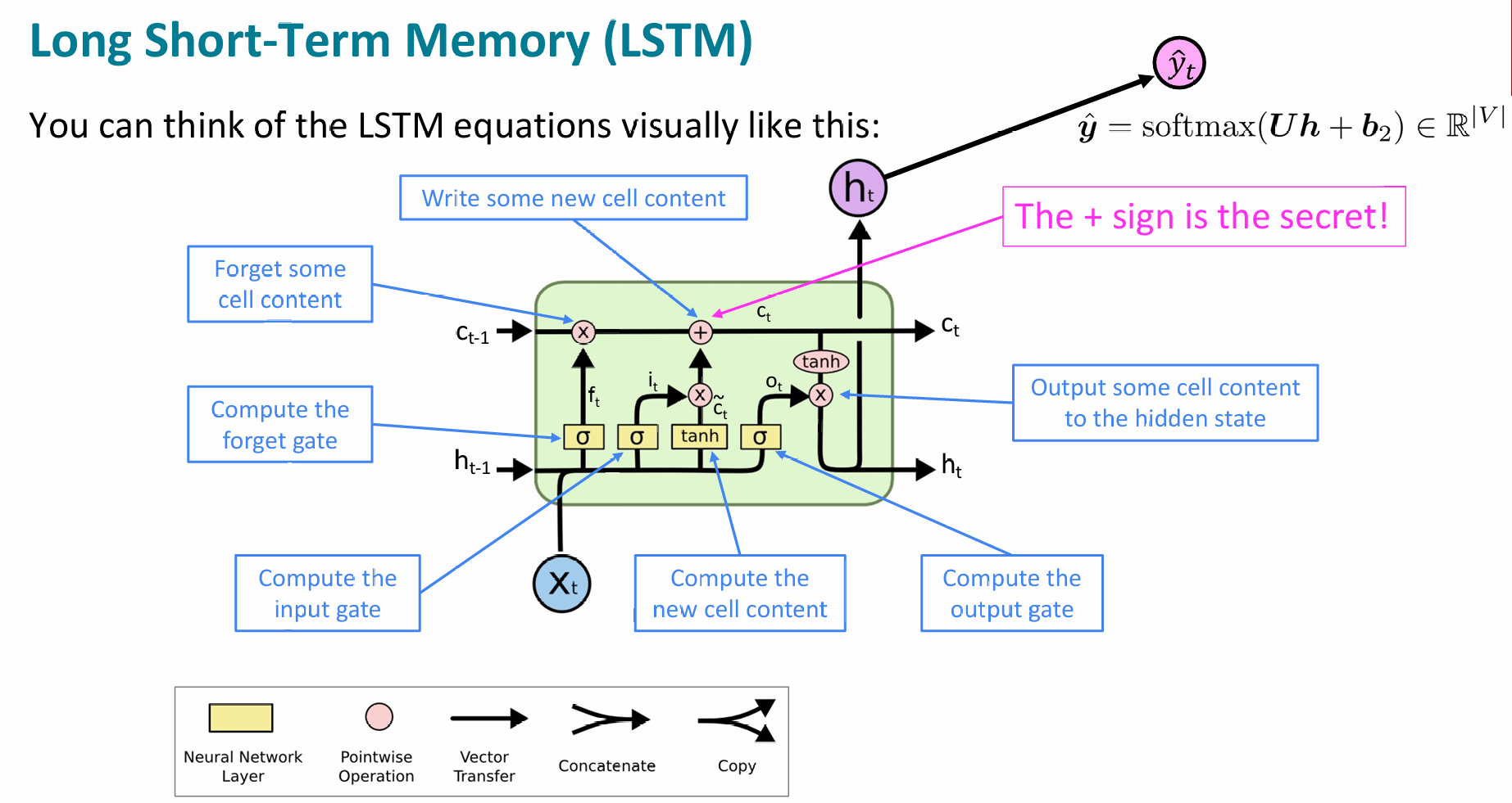
- In the figure above, each line carries a complete vector from one node’s output to other nodes’ inputs. Pink circles represent pointwise operations such as vector addition, and yellow boxes represent learned neural network layers. Merged lines represent concatenation, and forked lines mean the content is copied and sent to different places.
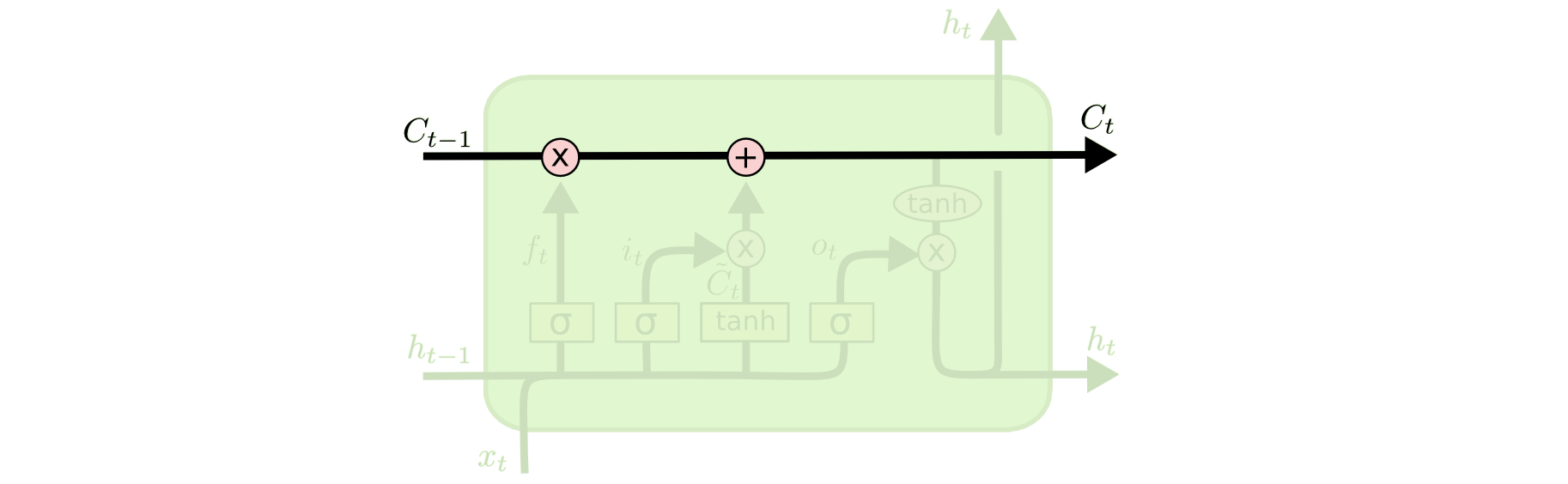
The key to LSTM is the cell state, the horizontal line running through the top of the diagram.
The cell state is like a conveyor belt. It runs straight through the chain with only minor linear interactions. Information can flow along it relatively unchanged.
LSTMs can add or remove information from the cell state. This is carefully controlled by structures called gates.
A gate is a way to selectively allow information through. It consists of a sigmoid neural network layer and a pointwise multiplication operation.
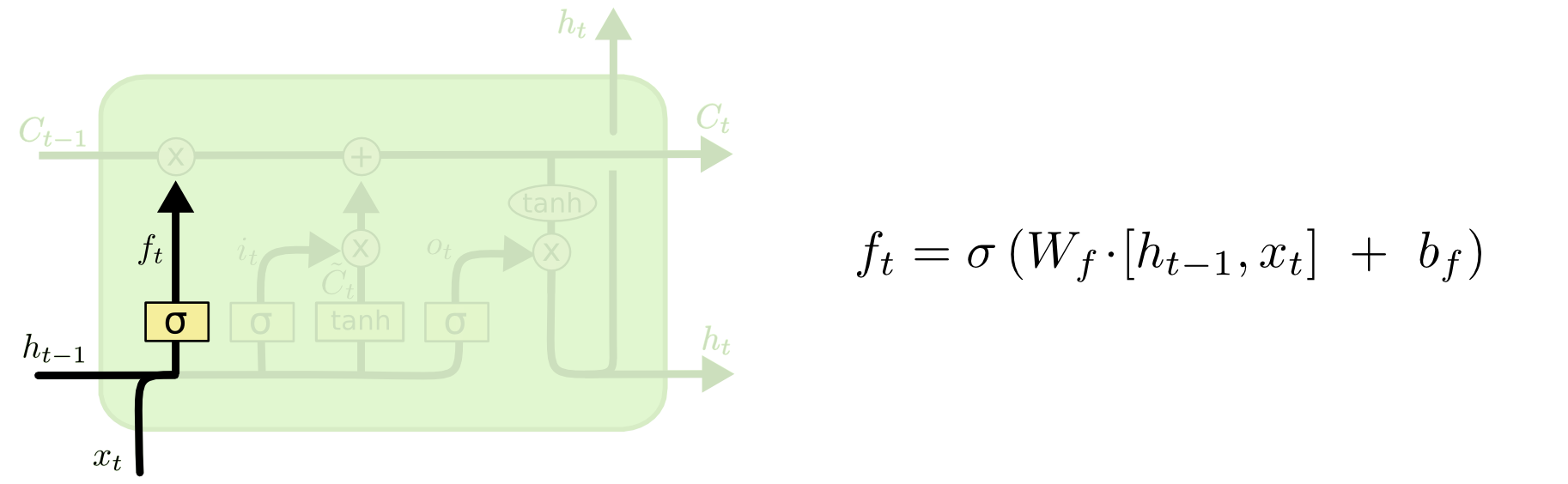
- The first step of an LSTM is to decide what information to discard from the cell state. This decision is made by the forget gate layer, a sigmoid layer. It receives $h_{t-1}$ and $x_t$, and outputs a value between 0 and 1 for each number in the previous cell state $C_{t-1}$. A value of 1 means “keep completely”; 0 means “discard completely”.
- Returning to the language-model example, the cell state may contain the gender of the current subject, so the model can use the correct pronoun. When a new subject appears, we want to forget the gender of the old subject.
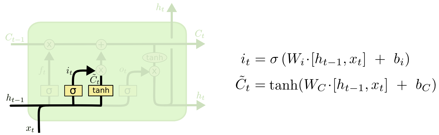
- The next step is to decide what new information to store in the cell state. This has two parts. First, an input gate layer decides which values to update. Then a $\tanh$ layer creates a vector of new candidate values $\tilde{C}_t$ that can be added to the state. In the next step, these two parts are combined to update the state.
- In the language-model example, we want to add the gender of the new subject into the cell state, replacing the old gender information we are forgetting.
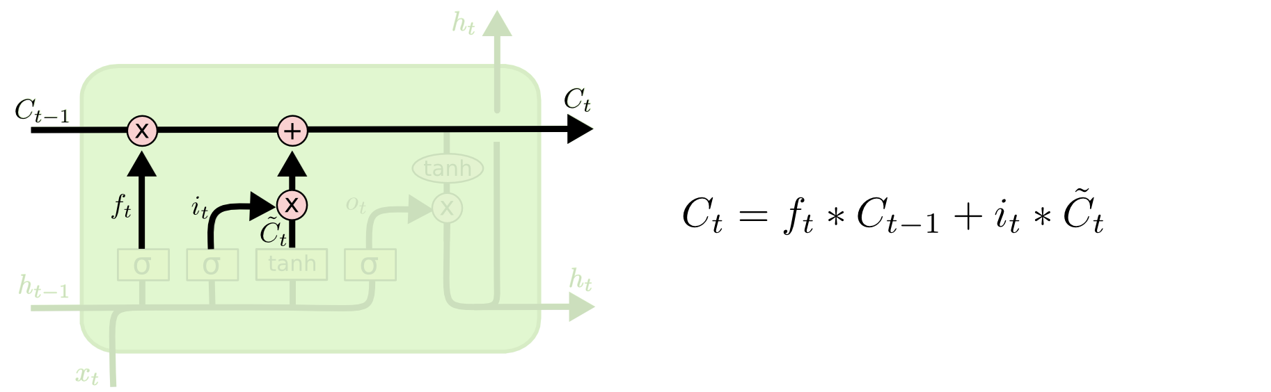
Now it is time to update the old cell state $C_{t-1}$ into the new cell state $C_t$. The previous steps already decided what to do; now we execute it.
We multiply the old state by $f_t$ to forget the information we decided to forget. Then we add $i_t * \tilde{C}_t$. These are the new candidate values, scaled by how much we decided to update each state value.
In the language-model example, this is where we actually remove the old subject-gender information and add the new information.
Finally, we need to decide what to output. This output is based on the cell state, but it is a filtered version.
First, we run a sigmoid layer to decide which parts of the cell state to output. Then we pass the cell state through $\tanh$, pushing values into the range -1 to 1, and multiply it by the sigmoid gate output. In this way, we only output the parts we decided to output.
In a language-model example, after processing a subject, the model may want to output information related to the upcoming verb, such as whether the subject is singular or plural.
How does LSTM solve vanishing gradients
The LSTM architecture makes it easier for an RNN to preserve information over multiple time steps. For example, if the forget gate of a cell dimension is set to 1 and the input gate is set to 0, that information can be kept indefinitely.
In contrast, a vanilla RNN must learn a recurrent weight matrix $W_h$ that preserves information in the hidden state, which is much harder.
Although vanishing and exploding gradients cannot be completely avoided, models can create more direct and more linear paths for long-distance dependencies. ResNet and DenseNet are examples of architectures that create direct connections between modules or layers.
Bidirectional RNNs
- Traditional one-way RNNs or LSTMs have an obvious limitation: when processing a sequence, they can only “look left”, meaning they only use past context. However, in many NLP tasks such as sentiment classification, named entity recognition, or sentence-level understanding, the meaning of the current word may also depend on the “right side”, or future context.
- To solve this, researchers introduced bidirectional architectures, often implemented with LSTMs:
- Forward RNN: processes the input sequence from left to right and computes hidden states $\overrightarrow{h}_t$.
- Backward RNN: processes the same input sequence from right to left and computes hidden states $\overleftarrow{h}_t$.
- Concatenated state: at each time step $t$, concatenate the forward and backward hidden states to form the final representation at that position: $h_t = [\overrightarrow{h}_t; \overleftarrow{h}_t]$. Each word representation therefore contains both left and right context.
- Bidirectional LSTMs are powerful feature extractors, but they are only suitable for tasks where the complete input sequence is available at once, such as text classification or encoding the source sentence in translation. They cannot be used for traditional language modeling, because language modeling predicts the next word. If the model can see future words on the right, it violates the autoregressive prediction setup.
Neural Machine Translation
- Neural machine translation was one of the first major successes of deep learning in NLP. NMT is mainly based on the Sequence-to-Sequence (Seq2Seq) architecture, whose core consists of two RNNs, usually LSTMs: an encoder and a decoder.
- The encoder reads the source-language sentence. While reading, it does not produce the translation directly; it continuously updates its hidden state. After the encoder processes the final word, its final hidden state is treated as a compressed semantic representation of the whole sentence. This acts as an “information bottleneck”, because all complex meanings of the source sentence must be compressed into one fixed-dimensional vector.
- The decoder-side LSTM is essentially a conditional language model. Its initial hidden state is not random or all zero; it is set to the bottleneck vector output by the encoder. This means every generation step of the decoder is conditioned on the semantic vector of the source sentence.
At each time step, it outputs the word with the highest probability according to the current hidden state, then feeds the last generated word into the next step until it produces the end-of-sentence token
<EOS>.