Data Mining Review
Content comes from PPTs and the key information highlighted at the end of the class.
Review Question PPT
What relationships does association rule mining in data mining primarily aim to discover between data items?
Association rule mining is mainly used to discover frequent co-occurrences or hidden associative relationships between data items.
In cluster analysis, what does the K value in the K-means algorithm represent?
In the K-means clustering algorithm, the K value represents the number of clusters the user expects the dataset to be partitioned into.
What algorithms exist for decision trees? What criteria do they mainly base their feature selection for partitioning on, and analyze the shortcomings of each criterion.
| Algorithm | Criterion | Shortcoming |
|---|---|---|
| ID3 | Information Gain | Strongly prefers multi-valued features, prone to overfitting |
| C4.5 | Information Gain Ratio | Computation is more complex, might prefer features with fewer values |
| CART | Gini Index | Has a slight preference for multi-valued features, tends towards unbalanced splits |
Given a simple text classification training set used to determine whether an email is “Spam”. The dictionary contains the following 5 words:
["deal", "money", "urgent", "meeting", "free"]
Training data:
- Spam (Spam, S):
- “deal free money”
- “urgent free deal”
- “money urgent free”
- Non-spam (Ham, H):
- “meeting deal”
- “urgent meeting”
The contents of the new email to be classified are: “free urgent meeting”
Task requirements: Use the multinomial Naive Bayes model (applying Laplace smoothing, where the smoothing parameter $\lambda=1$) to classify the email. Please complete the following calculations step-by-step:
Calculate the prior probabilities $P(Spam)$ and $P(Ham)$.
Total number of documents: $N_{\text{doc}} = 3 + 2 = 5$
$P(S) = \frac{3}{5} = 0.6$
$P(H) = \frac{2}{5} = 0.4$Prior probability results:
$P(S) = 0.6, \quad P(H) = 0.4$Calculate the class-conditional probability of each word under the Spam and Ham categories.
Dictionary size $|V| = 5$
Spam:
deal: 2, money: 2, urgent: 2, meeting: 0, free: 3
- Total number of words: $2+2+2+0+3 = 9$
- Denominator: $9 + 5 = 14$
$P(\text{deal}|S) = \frac{2+1}{14} = \frac{3}{14}$
$P(\text{money}|S) = \frac{2+1}{14} = \frac{3}{14}$
$P(\text{urgent}|S) = \frac{2+1}{14} = \frac{3}{14}$
$P(\text{meeting}|S) = \frac{0+1}{14} = \frac{1}{14}$
$P(\text{free}|S) = \frac{3+1}{14} = \frac{4}{14}$Ham:
deal: 1, money: 0, urgent: 1, meeting: 2, free: 0
Total number of words: $1+0+1+2+0 = 4$
Denominator: $4 + 5 = 9$
$P(\text{deal}|H) = \frac{1+1}{9} = \frac{2}{9}$
$P(\text{money}|H) = \frac{0+1}{9} = \frac{1}{9}$
$P(\text{urgent}|H) = \frac{1+1}{9} = \frac{2}{9}$
$P(\text{meeting}|H) = \frac{2+1}{9} = \frac{3}{9}$
$P(\text{free}|H) = \frac{0+1}{9} = \frac{1}{9}$Express the new email “free urgent meeting” as a term frequency vector.
Term frequency vector for “free urgent meeting” (in dictionary order: deal, money, urgent, meeting, free):
$[0, 0, 1, 1, 1]$Calculate the posterior probabilities of the email belonging to Spam and Ham.
Spam:
$P(S|d) \propto P(S) \times P(\text{urgent}|S) \times P(\text{meeting}|S) \times P(\text{free}|S)$
$= 0.6 \times \frac{3}{14} \times \frac{1}{14} \times \frac{4}{14}$
$= 0.6 \times \frac{12}{2744} \approx 0.002624$Ham:
$P(H|d) \propto P(H) \times P(\text{urgent}|H) \times P(\text{meeting}|H) \times P(\text{free}|H)$
$= 0.4 \times \frac{2}{9} \times \frac{3}{9} \times \frac{1}{9}$
$= 0.4 \times \frac{6}{729} \approx 0.003292$Normalization:
$P(S|d) = \frac{0.002624}{0.002624 + 0.003292} \approx 0.444$
$P(H|d) = \frac{0.003292}{0.002624 + 0.003292} \approx 0.556$Determine its final category based on the posterior probabilities.
Since $P(H|d) > P(S|d)$, the new email is classified as:
$\boxed{Ham}$
2.1.4 Types of Attributes
Nominal, Ordinal, Interval, Ratio
| Attribute Type | Description | Examples | Operations | |
|---|---|---|---|---|
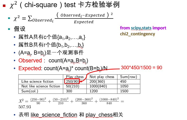
| Categorical (Qualitative) | Nominal | The values of a nominal attribute are just different names, meaning nominal values only provide enough information to distinguish objects (=, ≠) | Zip code, employee ID number, gender | Mode, entropy, contingency correlation, chi-square test |
| Ordinal | The values of an ordinal attribute provide enough information to determine the order of objects (<, >) | Ore hardness {good, average}, grade levels, street numbers | Median, percentiles, rank correlation, run test, sign test | |
| Numeric (Quantitative) | Interval | For interval attributes, the differences between values are meaningful, meaning a unit of measurement exists (+, -) | Calendar dates, Celsius or Fahrenheit temperatures | Mean, standard deviation, Pearson correlation coefficient, t and F tests |
| Ratio | For ratio attributes, both differences and ratios are meaningful (+, -, *, /) | Absolute temperature, monetary amounts, counts, age, mass, length, electrical current | Geometric mean, harmonic mean, percent variation |
2.2.1 Measures of Central Tendency
Mean, median, and mode
$Mean-mode = 3 * (mean - median)$
2.2.2 Interquartile Range
The first quartile, i.e., the data at the 25th percentile is $(n-1)/4$ (This is only for the first quartile; if it is the third quartile, it needs to be multiplied by 3).
If n is even, we need $+0.25\times (d_{n+1}-d_n)$ (This is only for the first quartile; if it is the third quartile, it’s 0.75).
2.4.4 Proximity Measures for Numeric Attributes
The Minkowski distance between two $p$-dimensional variables $x_1 = \{x_{11}, x_{12}, \ldots, x_{1p}\}$ and $x_2 = \{x_{21}, x_{22}, \ldots, x_{2p}\}$ is defined as:
$$ d(i,j) = \sqrt[q]{|x_{i1} - x_{j1}|^q + |x_{i2} - x_{j2}|^q + \cdots + |x_{ip} - x_{jp}|^q} $$When $q=1$, it represents the Manhattan distance:
$$ d(i,j) = |x_{i1} - x_{j1}| + |x_{i2} - x_{j2}| + \cdots + |x_{ip} - x_{jp}| $$When $q=2$, it represents the Euclidean distance:
$$ d(i,j) = \sqrt{|x_{i1} - x_{j1}|^2 + |x_{i2} - x_{j2}|^2 + \cdots + |x_{ip} - x_{jp}|^2} $$When $q \to \infty$, it represents the Chebyshev distance:
$$ d(i,j) = \lim_{q \to \infty} \left( \sum_{k=1}^p |x_{ik} - x_{jk}|^q \right)^{\frac{1}{q}} = \max_{1 \le k \le p} |x_{ik} - x_{jk}| $$n Euclidean and Manhattan distances satisfy the following mathematical properties
Positive definiteness: the distance is a non-negative number d(i,j)>0, if i≠j d(i,i)=0
Symmetry: d(i,j)=d(j,i)
Triangle inequality
2.4.8 Cosine Similarity
Cosine similarity can be used to compare the similarity of documents
$$ s(x, y) = \frac{x^T y}{\|x\|_2 \|y\|_2} \quad x = [1, 1, 0, 0] \quad y = [0, 1, 1, 0] $$$$ s(x, y) = \frac{0 + 1 + 0 + 0}{\sqrt{2} \sqrt{2}} = 0.5 $$3.2 Data Preprocessing
Data cleaning
- Fill in missing values, smooth noisy data, identify or remove outliers, and resolve inconsistencies
Data integration
- Integrate multiple databases, data cubes, or files
Data reduction
- Dimensionality reduction, data compression, Numerosity Reduction
Data transformation and data discretization
- Normalization
- Concept hierarchy generation
3.2.1 How to Handle Missing Data
- Ignore the tuple
- When the class label is missing, in supervised learning
- When the proportion of missing values for a specific attribute is large
- Manually fill in the missing value, which is computationally expensive
- Automatically fill in
- Use a global constant
- Use the attribute mean to fill in the missing value
- Global attribute mean
- Mean of the attribute for data objects belonging to the same class
- The most probable value: inference based on Bayesian formula or decision tree, regression, nearest neighbor strategy
3.2.4 Correlation Analysis
3.2.7 Data Reduction Strategies
Why perform data reduction?
Because a data warehouse can store terabytes of data, complex data analysis on a complete dataset may take a very long time.
Generally, data reduction is required during data preprocessing.
Replaces the original data with a smaller dataset.
Common data reduction strategies
Dimensionality reduction
Data reduction
Data compression
3.2.8 Dimensionality Reduction
- PCA (Principal Component Analysis) method
- Non-negative Matrix Factorization (NMF)
- Linear Discriminant Analysis (LDA)
Feature Selection
Select a representative subset of features from the original feature set
Single-feature importance evaluation
Model-based feature importance evaluation
3.2.11 Normalization
Min-Max Normalization
- Normalizes an attribute $A$ from interval $[\min_A, \max_A]$ to $[new_{\min_A}, new_{\max_A}]$ $$ v' = \frac{v - \min_A}{\max_A - \min_A} (new_{\max_A} - new_{\min_A}) + new_{\min_A} $$
- Example: Normalize income from the interval $12000$ to $98000$ to between $[0,1]$, what is the normalized value of $73600$?
Z-score Normalization
$$ v' = \frac{v - \mu_A}{\sigma_A} $$- Example: The mean of attribute $A$ is $\mu_A = 54000$, the standard deviation is $\sigma_A = 16000$, what is the normalized value of $73600$?
Decimal Scaling Normalization
- Move the position of the decimal point; the number of places to move depends on the maximum absolute value of attribute $A$, defined by the formula $$ v' = \frac{v}{10^j} $$
- $j$ is the smallest integer such that $\max(|v'|) < 1$
- For example: the minimum value of a dataset is $12000$, maximum value is $98000$, then the value of $j$ is $5$ $$ [12000, 98000] \rightarrow [0.12, 0.98] $$
4.3.2 Decision Tree Construction
- Decision Tree: A tree-like structured model learned from training data. It is a predictive analysis model expressed in the form of a tree structure (including binary trees and multi-way trees).
- A decision tree is a supervised learning algorithm and belongs to discriminative models.
- A decision tree is also known as a classification capability tree and is an important classification and regression method in data mining technology.
- There are two types of decision trees: classification trees and regression trees.
- Decision tree learning typically consists of 3 steps: feature selection, decision tree generation, and decision tree pruning.
- Commonly used methods: ID3, C4.5, CART
4.5 KNN Algorithm
- The k-Nearest Neighbor (kNN) method is a relatively mature and also the simplest machine learning algorithm, which can be used for basic classification and regression methods.
- The main idea of the algorithm: If a sample is most similar (i.e., its nearest neighbors in the feature space) to $k$ instances in the feature space, then whichever category the majority of these $k$ instances belong to, the sample will also belong to that category.
- Three fundamental elements of the $k$-nearest neighbor algorithm: the choice of $k$ value, distance metric, and classification decision rule.
Differences Between KNN and K-Means
K-NN is a classification algorithm in supervised learning where Categories are known. It trains and learns from classified data to find the features of these different classes, and then classifies unclassified data.
K-Means is a clustering algorithm in unsupervised learning. It is unknown beforehand how the data will be classified. Through cluster analysis, data is grouped into several clusters. Clustering doesn’t require training and learning over data.
Supervised Learning and Unsupervised Learning
Supervised learning is a machine learning method which utilizes labeled data for training. Every input data has a corresponding output label, and the model predicts by learning the relationship between these inputs and outputs.
Characteristics:
Requires extensive labeled data.
The training process has a definite objective, and the model can continuously adjust through feedback.
Common algorithms include linear regression, logistic regression, support vector machines (SVM), decision trees, etc.
Application Scenarios:
- Suitable for classification and regression problems, such as image recognition, speech recognition, and financial forecasting.
Unsupervised learning is a machine learning method in which training is performed using unlabeled data. The model automatically discovers patterns and structures from the input data without relying on any labels.
- Characteristics:
- Does not require labeled data, making it suitable for processing large amounts of unlabeled data.
- The training process lacks an explicit goal; the model learns through the intrinsic structure of the data.
- Common algorithms include clustering (e.g., K-Means), association rule learning (e.g., Apriori algorithm), etc.
- Application Scenarios:
- Suitable for data clustering, market segmentation, anomaly detection, etc.
5.3 Density-Based Clustering Methods
DBSCAN Algorithm Description
Input: A database containing $n$ objects, radius $\varepsilon$ (Eps), and minimum number MinPts
Output: All generated clusters that meet density requirements
Repeat
- Extract an unprocessed point from the data
- If the extracted point is a core point Then find all objects density-reachable from this point to form a cluster
- Else the extracted point is a border point (non-core object), exit the current iteration, and seek the next point
- EndIf
Until all points are processed
Core object: If the $\varepsilon$-neighborhood of an object contains at least a minimum number of objects, MinPts, the object is called a core object.
A border point’s “Eps” ($\varepsilon$) neighborhood contains fewer than MinPts objects, but a core object exists within its neighborhood.
6.1 Confusion Matrix
Confusion Matrix
| Actual Class \ Predicted Class | Class=Yes | Class=No |
|---|---|---|
| Class=Yes | a (TP) | b (FN) |
| Class=No | c (FP) | d (TN) |
- $a+d$ represents the number of correctly classified samples among all samples
- $b+c$ represents the number of incorrectly classified samples among all samples
- $a+b+c+d$ represents the total number of samples
- Accuracy
Recall
$$ recall = \frac{TP}{TP+FN} $$- Represents the proportion of positive samples that are correctly predicted, that is, how many positive samples are correctly identified.
Precision
$$ precision = \frac{TP}{TP+FP} $$- Represents the proportion of truly positive samples out of those predicted as positive, that is, how many of the predicted true sample predictions are actually correct positive.
6.5 Overfitting and Underfitting
Causes of Overfitting:
Noise: The training set contains a massive volume of noisy data.
Lack of representative samples: The size of the training set is comparatively small, resulting in overly complex training models.
7.1 Advantages of Ensemble Learning
Can effectively reduce prediction error
Suppose an ensemble classifier consists of 3 individual classifiers, where the error rate of each classifier is 40%. Let C denote a correct prediction, I denote an incorrect prediction, and Probability denote the probability of the final prediction result. The total number of combinations is $2^3=8$.
The model’s error rate is: 0.096+0.096+0.096+0.064=35.2% < 40%
Let the number of models be $m$, and the error rate of each model be $r$.
The general formula for calculating error is:
$$ p(error) = \sum_{i=(m+1)/2}^{m} C_{m}^{i} r^{i}(1-r)^{m-i} $$- When over half of the $m$ models misclassify -> the final result is wrong, $i$ ranges from $(m+1)/2$ to $m$.
- Randomly selecting $i$ out of $m$, the remaining $m-i$ models classify correctly.
- The figure below depicts the relations between error rates and model scales when $r=0.4$.