References

自学SQL网(教程 视频 练习全套)

Learn the knowledge and immediately have exercises to do.

MySQL 教程 | 菜鸟教程

MySQL总结_sq连表-CSDN博客

主键 - SQL教程 - 廖雪峰的官方网站

Best viewing experience tutorial.

Relational Model

Quoted from 关系模型 - SQL教程 - 廖雪峰的官方网站

Primary Key

In a relational database, each row of data in a table is called a record. A record is composed of multiple fields. For example, two records in the students table:

For a relational table, there is a very important constraint: any two records cannot be duplicated. Non-duplication doesn’t mean two records are not entirely identical, but rather that different records can be uniquely distinguished by a certain field, and this field is called the primary key.

For example, assuming we use the name field as the primary key, then we can uniquely identify a record through the name Xiaoming or Xiaohong. However, with this setup, we couldn’t store students with the same name, because inserting two records with the same primary key is not allowed.

The most crucial requirement for a primary key is: once a record is inserted into the table, it’s best not to modify the primary key anymore, because the primary key is used to uniquely locate a record. Modifying the primary key will cause a series of cascading effects.

Because the role of the primary key is so important, how to select a primary key will have a significant impact on business development. If we use a student’s ID number as the primary key, it seems to uniquely locate a record. However, an ID number is also a business scenario. If the ID number’s length increases or needs to be changed, and as a primary key, it has to be modified, it will have a severe impact on the business.

Therefore, a basic principle for selecting a primary key is: do not use any business-related fields as the primary key.

Thus, fields that seem unique like ID numbers, mobile phone numbers, and email addresses, should not be used as primary keys.

The best primary key is a field completely unrelated to the business, and we generally name this field id. Common types suitable for the id field are:

1. Auto-incrementing integer type: The database will automatically assign an auto-incrementing integer to each record upon insertion, so we don’t have to worry at all about primary key duplication, nor do we need to pre-generate the primary key ourselves;
2. Globally Unique Identifier (GUID) type: Also known as UUID, using a globally unique string as a primary key, such as 8f55d96b-8acc-4636-8cb8-76bf8abc2f57. The GUID algorithm ensures that the strings generated by any computer at any time are different through network card MAC addresses, timestamps, and random numbers. Most programming languages have built-in GUID algorithms, allowing you to pre-calculate the primary key.

For most applications, an auto-incrementing primary key is usually sufficient. The primary key we defined in the students table is also of BIGINT NOT NULL AUTO_INCREMENT type.

If an INT auto-increment type is used, an error will occur when the number of records in a table exceeds 2,147,483,647 (about 2.1 billion) as it reaches the upper limit. Using the BIGINT auto-increment type allows for a maximum of about 9.22 quintillion records.

Summary

The primary key is the unique identifier for a record in a relational table. Selecting a primary key is very important: a primary key should not have any business meaning, and should instead use a BIGINT auto-increment or GUID type. A primary key should also not allow NULL.

Multiple columns can be used as a composite primary key, but composite primary keys are not commonly used.

Foreign Key

When we uniquely identify records using a primary key, we can determine any student’s record in the students table:

We can also determine any class record in the classes table:

But how do we determine which class a record in the students table belongs to, for example, Xiaoming with id=1?

Since one class can have multiple students, in the relational model, the relationship between these two tables can be called “one-to-many”, meaning one record in the classes table can correspond to multiple records in the students table.

To express this one-to-many relationship, we need to add a class_id column to the students table, letting its value correspond to a specific record in the classes table:

This way, we can directly locate which record in the classes table a students table record should correspond to based on the class_id column.

• Xiaoming’s class_id is 1, therefore, the corresponding record in the classes table is Class 1 with id=1;
• Xiaohong’s class_id is 1, therefore, the corresponding record in the classes table is Class 1 with id=1;
• Xiaobai’s class_id is 2, therefore, the corresponding record in the classes table is Class 2 with id=2.

In the students table, through the class_id field, data can be associated with another table, and such a column is called a foreign key.

A foreign key is not implemented through the column name, but by defining a foreign key constraint:

1
2
3
4

ALTER TABLE students
ADD CONSTRAINT fk_class_id
FOREIGN KEY (class_id)
REFERENCES classes (id);

Here, the foreign key constraint name fk_class_id can be anything, FOREIGN KEY (class_id) specifies class_id as the foreign key, and REFERENCES classes (id) specifies that this foreign key will be linked to the id column of the classes table (i.e., the primary key of the classes table).

By defining a foreign key constraint, a relational database can guarantee that invalid data cannot be inserted. That is, if a record with id=99 doesn’t exist in the classes table, the students table cannot insert a record with class_id=99.

Since foreign key constraints reduce database performance, most Internet applications, in pursuit of speed, do not set foreign key constraints and solely rely on the application itself to ensure logical correctness. In this case, class_id is just an ordinary column, it simply acts as a foreign key.

To delete a foreign key constraint, it is also achieved via ALTER TABLE:

1
2

ALTER TABLE students
DROP FOREIGN KEY fk_class_id;

Note: Deleting a foreign key constraint does not delete the foreign key column itself. Deleting a column is achieved via DROP COLUMN ....

Many-to-Many

By associating a foreign key in one table with another table, we can define a one-to-many relationship. Sometimes, we also need to define a “many-to-many” relationship. For example, one teacher can correspond to multiple classes, and one class can also correspond to multiple teachers. Thus, there is a many-to-many relationship between the class table and the teacher table.

A many-to-many relationship is actually implemented through two one-to-many relationships. That is, by using an intermediate table to connect two one-to-many relationships, a many-to-many relationship is formed:

teachers table:

classes table:

Intermediate table teacher_class connecting two one-to-many relationships:

Through the intermediate table teacher_class, we can know the relationship from teachers to classes:

• Mr. Zhang with id=1 corresponds to Class 1 and Class 2 with id=1,2;
• Mr. Wang with id=2 corresponds to Class 1 and Class 2 with id=1,2;
• Mr. Li with id=3 corresponds to Class 1 with id=1;
• Mr. Zhao with id=4 corresponds to Class 2 with id=2.

Similarly, we can know the relationship from classes to teachers:

• Class 1 with id=1 corresponds to Mr. Zhang, Mr. Wang, and Mr. Li with id=1,2,3;
• Class 2 with id=2 corresponds to Mr. Zhang, Mr. Wang, and Mr. Zhao with id=1,2,4;

Therefore, through the intermediate table, we’ve defined a “many-to-many” relationship.

One-to-One

A one-to-one relationship means that a record in one table corresponds to a single, unique record in another table.

For instance, every student in the students table can have their own contact information. If we store the contact details in another table contacts, we can obtain a “one-to-one” relationship:

Some attentive readers might ask, since it’s a one-to-one relationship, why not just add a mobile column to the students table so they can be merged into one?

If the business logic allows, combining the two tables into one is entirely possible. However, sometimes if a student doesn’t have a mobile number, a corresponding record wouldn’t exist in the contacts table. In fact, a one-to-one relationship, strictly speaking, is the contacts table having a one-to-one correspondence with the students table.

Furthermore, some applications split a large table into two one-to-one tables to separate frequently read fields from infrequently read ones for better performance. For example, splitting a large user table into a basic user information table user_info and a detailed user information table user_profiles. Most of the time, only the user_info table needs to be queried without querying user_profiles, which improves the query speed.

Summary

Relational databases can implement one-to-many, many-to-many, and one-to-one relationships using foreign keys. Foreign keys can either be constrained by the database or set without constraints, relying solely on the application’s logic to guarantee integrity.

Index

In a relational database, if there are tens of thousands or even hundreds of millions of records, you need to use indexes to achieve very fast query speeds.

An index is a strictly pre-sorted data structure in a relational database for the values of one or multiple columns. By utilizing indexes, the database system doesn’t have to scan the entire table, but directly pinpoints the records that meet the criteria, greatly speeding up queries.

For example, for the students table:

If you frequently query based on the score column, you can create an index on the score column:

1
2

ALTER TABLE students
ADD INDEX idx_score (score);

Using ADD INDEX idx_score (score) creates an index named idx_score that utilizes the score column. The index name is arbitrary, and if the index comprises multiple columns, they can be written sequentially in parentheses, for example:

1
2

ALTER TABLE students
ADD INDEX idx_name_score (name, score);

The efficiency of an index depends on whether the values of the indexed column are dispersed—that is, the more distinct the column’s values are, the higher the index efficiency. Conversely, if a column’s records contain a large number of identical values, like the gender column where roughly half the values are M and the other half are F, creating an index for that column makes no sense.

You can create multiple indexes for a single table. The advantage of indexes is improved query efficiency, while the disadvantage is that when inserting, updating, and deleting records, the index needs to be modified simultaneously. Therefore, the more indexes there are, the slower the operations to insert, update, and delete records become.

For primary keys, relational databases will automatically create a primary key index for them. Using a primary key index is the most efficient because the primary key guarantees absolute uniqueness.

Unique Index

When designing relational data tables, columns that appear unique, such as ID numbers and email addresses, should not be modeled as primary keys due to having business significance.

However, based on business requirements, these columns still have a uniqueness constraint: meaning two records cannot store the exact same ID number. At this point, we can add a unique index to this column. For example, assuming the name in the students table cannot be duplicated:

1
2

ALTER TABLE students
ADD UNIQUE INDEX uni_name (name);

Through the UNIQUE keyword, we have added a unique index.

You can also add a unique constraint to a certain column without creating a unique index:

1
2

ALTER TABLE students
ADD CONSTRAINT uni_name UNIQUE (name);

In this scenario, the name column doesn’t have an index, but still maintains a uniqueness guarantee.

Regardless of whether an index is created or not, using a relational database will make no difference to the user and the application. This implies that when we query the database, if a matching index is available, the database system will automatically utilize the index to boost query efficiency. If no index exists, the query will still execute normally, but at a slower speed. Hence, indexes can be progressively optimized during database usage.

Summary

Creating indexes for database tables can accelerate query speeds;

Creating unique indexes acts to guarantee the uniqueness of the values in a specific column;

Database indexes are transparent to both users and applications.

SELECT Query

1
2
3
4
5
6
7
8

SELECT column, another_column, …
FROM mytable
WHERE condition
    AND/OR another_condition
    AND/OR …;
    
SELECT * FROM movies 
WHERE year>=2010 AND length_minutes<120;

Filtering Numeric Attribute Columns

Filtering String Attribute Columns

1
2
3
4
5
6
7

/* Wildcards */
col_name LIKE "%AT%";
/* "AT", "AT*...", "...*AT", "...*AT*..." all satisfy the condition
 There can be arbitrary characters before and after "AT" */
col_name LIKE "AN_";
/* "AND" is okay, "AN", "ANDD" are not
 Similar to '%', but only represents a single character */

Filtering / Sorting

1
2
3
4

/* Use the DISTINCT keyword to specify that a certain attribute column or columns return uniquely */
SELECT DISTINCT column, another_column, …
FROM mytable
WHERE condition(s);

 1
 2
 3
 4
 5
 6
 7
 8
 9
10
11

/* Sort the results based on one or more attribute columns */
SELECT column, another_column, …
FROM mytable
WHERE condition(s)
/* ASC for ascending or DESC for descending */
ORDER BY column ASC/DESC
/* LIMIT specifies how many rows of results to return
 OFFSET specifies from which row to start returning */
LIMIT num_limit OFFSET num_offset;
/* Regarding OFFSET, if you want to output the Nth row (and onwards)
 the parameter for OFFSET must be N-1 */

Example Problem

SELECT Review Problems

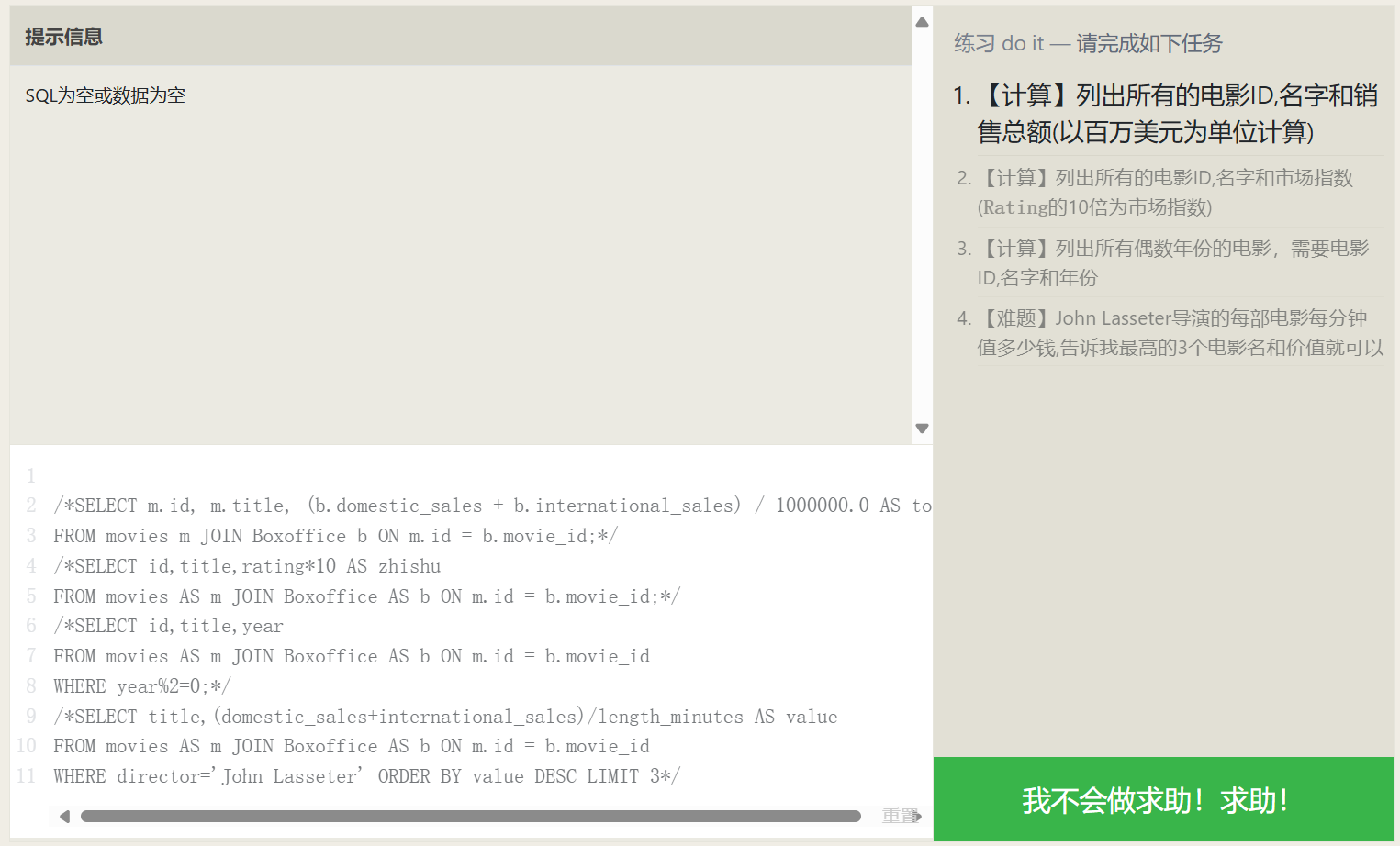
Using Expressions in Queries

Actually, AS is not only used for assigning aliases to expressions; standard attribute columns and even tables can be assigned an alias, making the SQL easier to grasp.

1
2
3
4
5

-- Examples of aliasing attribute columns and tables
SELECT column AS better_column_name, …
FROM a_long_widgets_table_name AS mywidgets
INNER JOIN widget_sales
  ON mywidgets.id = widget_sales.widget_id;

1
2
3
4
5

-- Example containing an expression
SELECT  particle_speed / 2.0 AS half_particle_speed -- Divided the results by 2
FROM physics_data
WHERE ABS(particle_position) * 10.0 >500
            -- (The condition requires the absolute value of this attribute multiplied by 10 to be greater than 500);

Performing Statistics in Queries

1
2
3

SELECT AGG_FUNC(column_or_expression) AS aggregate_description, …
FROM mytable
WHERE constraint_expression;

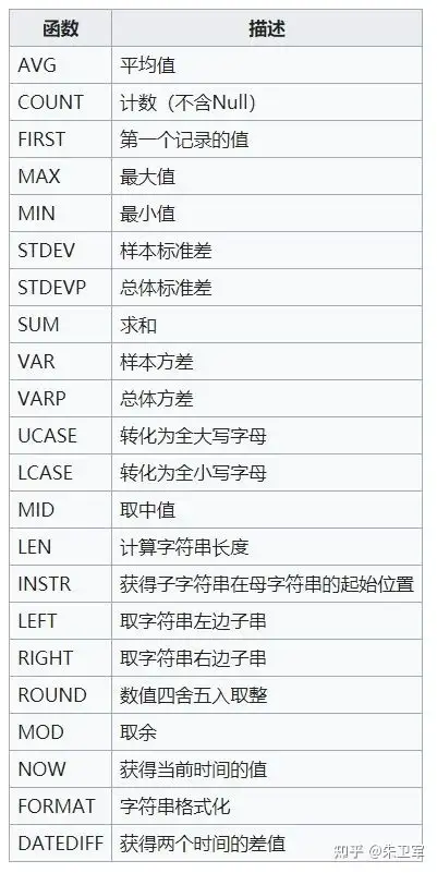
Common statistical functions:

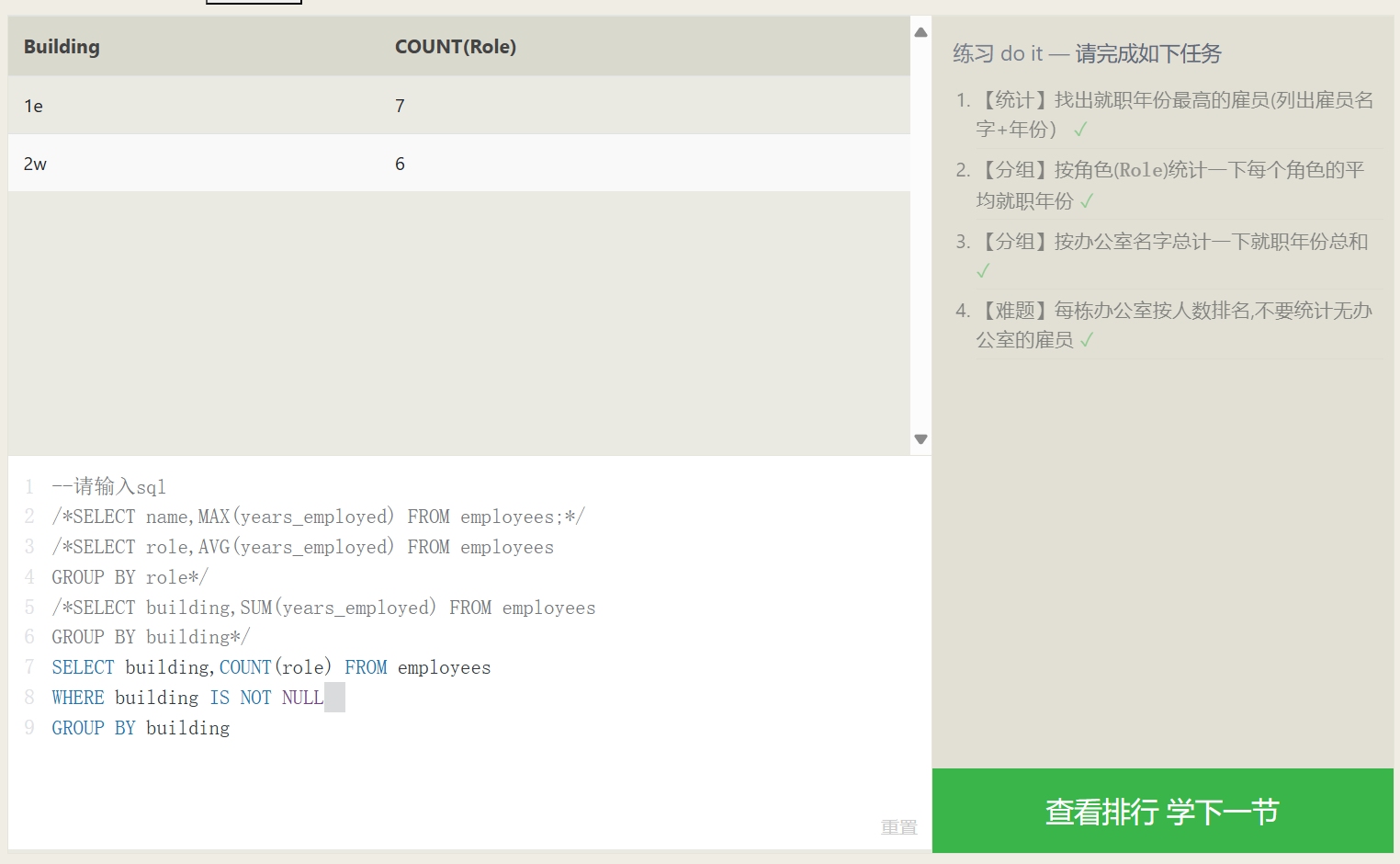
Grouped Statistics

The GROUP BY data grouping syntax can group data by a specific col_name. For example, GROUP BY Year means grouping the data by year, placing data from the same year into the same group. If a statistical function is combined with GROUP BY, then the statistical result is constrained to the data within each group. The number of data rows resulting from a GROUP BY grouping is exactly the number of groups. For instance, with GROUP BY Year, however many years exist in the overall data, that same number of data rows will be returned, regardless of whether a statistical function is applied.

1
2
3
4
5

-- Statistics using groupings
SELECT AGG_FUNC(column_or_expression) AS aggregate_description, …
FROM mytable
WHERE constraint_expression
GROUP BY column;

In the GROUP BY grouping syntax, we know that the database first filters the data with WHERE, and then groups the results. What if we want to filter out a few more rows from the already grouped data? A less commonly utilized syntax, the HAVING syntax, will be employed to resolve this problem; it allows further SELECT filtering on the post-grouping data.

The HAVING syntax is identical to WHERE, except the result set it operates on is different. In the case of the small datasets in our examples, HAVING may not seem very useful, but when your data volume hits the thousands or millions with numerous attributes, it can be of immense help.

JOIN Connections

Database Normal Forms

Database normal forms are standardizations for data table design. Under these normal form guidelines, the duplicate data stored by each schema is reduced to a minimum (assisting in maintaining data coherence). Meanwhile, under database normalization, tables no longer possess rigid data decoupling, permitting independent scaling (i.e., for example, the growth of car engines and cars is completely decoupled).

1
2
3
4
5
6
7
8

SELECT column, another_table_column, …
FROM mytable -- The primary table
INNER JOIN another_table -- The table to be joined
    ON mytable.id = another_table.id 
    -- Imagine the primary key join mentioned earlier, two identical ones are merged into 1 row
WHERE condition(s)
ORDER BY column, … ASC/DESC
LIMIT num_limit OFFSET num_offset;

The relation association described by the ON condition in this example:

INNER JOIN (Inner) Connections

First, combine the data from two tables together, any data from either table that fails to find a counterpart via ID will be discarded. At this stage, you may envision the post-join data as an aggregation of two tables, where the remaining SQL clauses will continue their execution upon this combination (imagine it’s exactly the same as the previous single-table operations). Another method for comprehending an INNER JOIN is to think of an INNER JOIN as the intersection of two sets.

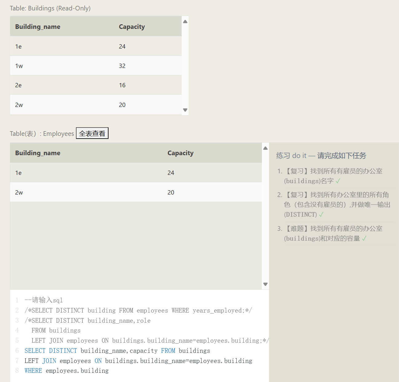
OUTER JOIN Outer Connections

1
2
3
4
5
6
7
8

-- Perform multi-table queries using LEFT/RIGHT/FULL JOINs
SELECT column, another_column, …
FROM mytable
INNER/LEFT/RIGHT/FULL JOIN another_table
    ON mytable.id = another_table.matching_id
WHERE condition(s)
ORDER BY column, … ASC/DESC
LIMIT num_limit OFFSET num_offset;

When executing a connection on Table A to Table B, a LEFT JOIN retains all elements of A, unaffected by if they match successfully with B, conversely, a RIGHT JOIN retains all elements present inside B. Concluding, a FULL JOIN will simultaneously conserve all row items originating from both A and B regardless of achieving any matches.

Establishing a 1-to-1 linkage connecting two table schemas reserves A’s or B’s intrinsic entries, where if a provided column doesn’t reside within the opposite table, a NULL is to fill up the consequential data.

Query Execution Order

 1
 2
 3
 4
 5
 6
 7
 8
 9
10

-- This is the complete SELECT query
SELECT DISTINCT column, AGG_FUNC(column_or_expression), …
FROM mytable
    JOIN another_table
      ON mytable.column = another_table.column
    WHERE constraint_expression
    GROUP BY column
    HAVING constraint_expression
    ORDER BY column ASC/DESC
    LIMIT count OFFSET COUNT;

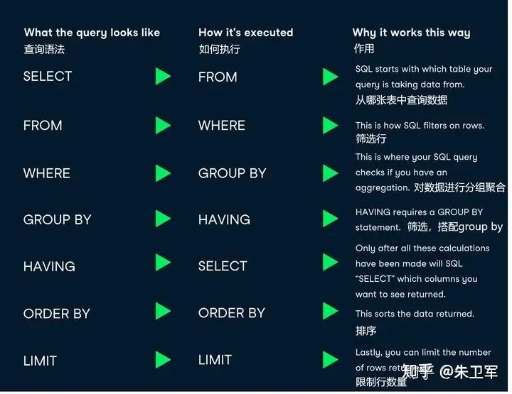
1. FROM and JOIN

FROM or JOIN are the first to execute, pinpointing the overall constraints behind a data range. Should different tables require a JOIN, an intermediate temporary Table may generate, subsequently serving later downstream operations. Fundamentally, this initial block could be summarized as recognizing the genesis data source table (inclusive of any temp tables).

2. WHERE

Now that we have ascertained the data schema source, the WHERE statement undertakes data screening on this data origin depending exclusively on specified parameters, ejecting whichever data entries do not correspond to the requested qualifications. All screened col attributes ought to materialize out of the tables identified through FROM. Due to aliases plausibly embodying non-executed formulas, AS aliases cannot be invoked dynamically inside this specific phase.

3. GROUP BY

If you implemented GROUP BY for classifying entries, the subsequent GROUP BY groups earlier data alongside computations for tallies, shrinking resultant outcomes aligned closer to the aggregate number of partitions. Therefore, any extra parameters not part of the classified dimensions get wiped.

4. HAVING

If you implemented GROUP BY clustering, HAVING conducts additional sifting onto corresponding outcome schemas immediately after finishing earlier groupings. AS aliases conversely stay deactivated for use amidst this procedure phase.

5. SELECT

After finalizing findings, SELECT is implemented across columns comprising the solution output to perform simple sifting operations or computational mathematics aimed specifically at establishing the explicit contents outputted.

6. DISTINCT

Should elements suffer uninvited repetition, DISTINCT bears the duty to enforce deduplication.

7. ORDER BY

Where the generated finding bounds stay solidly solidified, ORDER BY categorizes sequence alignments over the end-product. Since standard evaluation across variables enveloped in SELECT rests fulfilled. Thus here entails dynamic utility via establishing AS aliases.

8. LIMIT / OFFSET

As the conclusion steps, LIMIT beside OFFSET carve out compartmental slices directly abstracted right after sorted listings.

Conclusion

Not absolutely every SQL statement relies intrinsically around comprehensively capturing all potential terminologies, but nimbly navigating via varied compositional constructs paired securely closely with intuitive SQL theoretical execution foundations ensures superior resolutions handling localized database hurdles exclusively bounded natively on SQL, rather than blindly migrating all problematic dilemmas towards application code programming abstractions.

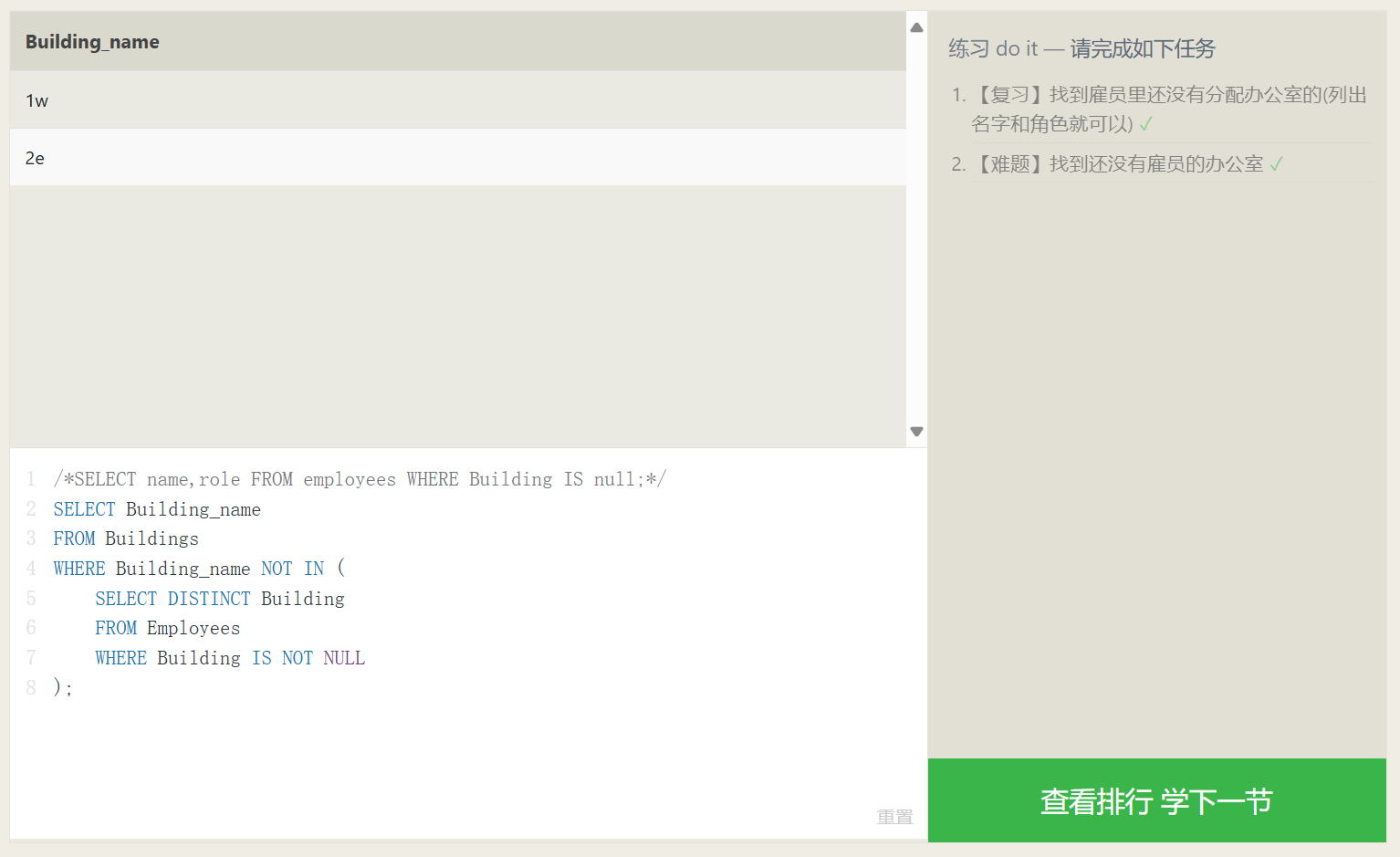
NULL

If you overlook committing distinct inputs allocated for designated database columns, it prominently projects a NULL. Thus, a recurrent solution allocates structural default values, typically like standardizing numeric fields to 0, combined with calibrating textual dimensions matching "" string dimensions. Nevertheless, where intrinsic characteristics authentically mirror absolute intentional NULL meanings, please pay cautious consideration against recklessly standardizing alternative defaults versus legitimately accepting pure NULL. (For example, whilst establishing cross-record average arithmetic, applying 0 automatically registers evaluations consequently contaminating accurate calculations, although deploying pure NULL exclusively bypasses erroneous quantitative inclusions entirely).

Another situational bracket proving highly restrictive preventing NULL generations involves executing outer-joining multi-schema combinations earlier narrated, considering whenever quantitative data discrepancies present amongst A contrasting B schemas, one absolutely depends directly around NULL to seamlessly patch up dimensions natively missing references. Tackling equivalent predicaments, manipulating logic gates bounded internally with IS NULL identically accompanied by IS NOT NULL expertly determines specific boolean verifications judging if a definitive spatial coordinate explicitly registers fundamentally parallel corresponding precisely toward NULL.

1
2
3
4
5

SELECT column, another_column, …
FROM mytable
WHERE column IS/IS NOT NULL
AND/OR another_condition
AND/OR …;

Modifying Data

Partially quoted from 修改数据 - SQL教程 - 廖雪峰的官方网站

The bedrock operational foundations revolving around relational database constructs categorically parallel CRUD manipulations: Create, Retrieve, Update, Delete. Addressing specific interrogations, we comprehensively expounded exactly describing elaborate dynamic utilities encompassing the SELECT statements effectively.

Transitioning precisely over dimensional expansions, excisions alongside modifications dynamically reflect parallel standard matching respective descriptive SQL queries:

• INSERT: Inject original fresh record items;
• UPDATE: Overwrite formerly registered content;
• DELETE: Terminate and rip historical documented dimensions out.

We will singularly unpack distinct structural application semantics independently driving these tri-fold modifying algorithmic assertions consecutively.

INSERT Insertion

Referenced in MySQL 插入数据 | 菜鸟教程

For illustration, injecting completely novel unrepresented components directly supplementing an internal user structural matrix primarily lists requisite sequential locational destinations dynamically accompanied by parallel structured inputs categorically sequentially encoded straightly following downstream VALUES parameters:

1
2
3
4
5

INSERT INTO table_name (column1, column2, column3, ...)
VALUES (value1, value2, value3, ...);
--
INSERT INTO users (username, email, birthdate, is_active)
VALUES ('test', 'test@runoob.com', '1990-01-01', true);

Whenever attempting holistic whole scale broad injections globally accommodating all columns (which ultimately equates loading literal standalone rows natively), explicit dimensional coordinates remain perfectly dismissible entirely voluntarily:

1
2

INSERT INTO users
VALUES (NULL,'test', 'test@runoob.com', '1990-01-01', true);

Moreover it is similarly trivial establishing multifaceted multi-tier simultaneous bundled row records entirely unified through simply assigning combined aggregated sets grouped intrinsically under VALUES clauses, sequentially mapping individualized items cleanly compartmentalized bound uniquely using encapsulated parenthesis formatted like (...) neatly divided employing systematic commas , effectively:

1
2
3
4
5

INSERT INTO users (username, email, birthdate, is_active)
VALUES
    ('test1', 'test1@runoob.com', '1985-07-10', true),
    ('test2', 'test2@runoob.com', '1988-11-25', false),
    ('test3', 'test3@runoob.com', '1993-05-03', true);

UPDATE Undergoing Updates

MySQL UPDATE 更新 | 菜鸟教程

1
2
3

UPDATE table_name
SET column1 = value1, column2 = value2, ...
WHERE condition;

Parameter Details:

• table_name is the name of the table wherein data rests scheduled anticipating functional updates.
• column1, column2, … highlight discrete positional columns formally recognized awaiting modifications outright.
• value1, value2, … outline structurally novel information intrinsically scheduled effectively overwriting earlier dated legacy materials seamlessly.
• WHERE condition represents conditional non-mandatory clauses functionally singling filtering parameters strictly governing explicitly updated rows. Omitting completely identical WHERE clauses subsequently universally upgrades holistically comprehensive tables unconditionally totally.

Complementary Additions:

• You remain effectively legally permitted upgrading independently singular and synchronously mixed multifield properties jointly.
• You seamlessly retain liberties programming absolutely disparate multifaceted conditions freely enveloped universally underneath WHERE subqueries.
• You natively manage comprehensive wide-scale adjustments immediately localized purely isolated targeting standalone tables independently.

Implementing conditional bounds effectively anchored via WHERE structures provides phenomenally irreplaceable instrumental control purposefully identifying discrete unique tabular boundaries specifically designated requiring surgical alterations effectively.

1
2
3
4

-- Update the value of a single column
UPDATE employees
SET salary = 60000
WHERE employee_id = 101;

1
2
3
4

-- Update the values of multiple columns
UPDATE orders
SET status = 'Shipped', ship_date = '2023-03-01'
WHERE order_id = 1001;

1
2
3
4

-- Use an expression to update a value
UPDATE products
SET price = price * 1.1
WHERE category = 'Electronics';

1
2
3
4
5
6
7
8

-- Update using a value from a subquery
UPDATE customers
SET total_purchases = (
    SELECT SUM(amount)
    FROM orders
    WHERE orders.customer_id = customers.customer_id
)
WHERE customer_type = 'Premium';

While authentically negotiating functionally operational structured rational core relational database engines like specifically MySQL inherently, deploying UPDATE statements generally consistently echoes feedback indicating successfully modified elements matching corresponding filtering parameters aligned alongside comprehensive WHERE clauses.

Showcasing structural examples, notably modernizing distinct elements bound identifying primarily tracking id=1 exactly natively:

1
2
3

mysql> UPDATE students SET name='大宝' WHERE id=1;
Query OK, 1 row affected (0.00 sec)
Rows matched: 1  Changed: 1  Warnings: 0

MySQL distinctly natively signals explicit responsive 1, transparently immediately visible inspecting completely rendered identical results cleanly reading Rows matched: 1 Changed: 1 accurately unequivocally.

Should corresponding updates primarily affect tracking exclusively registering elements possessing intrinsically tracking id=999 similarly:

1
2
3

mysql> UPDATE students SET name='大宝' WHERE id=999;
Query OK, 0 rows affected (0.00 sec)
Rows matched: 0  Changed: 0  Warnings: 0

MySQL naturally natively signifies respective conditional returning 0, explicitly transparently visible natively inspecting distinctly echoing outputs explicitly validating Rows matched: 0 Changed: 0 accurately clearly.

DELETE Removal

Basic fundamental grammar orchestrating structured DELETE syntaxes structurally aligns identically resembling:

1

DELETE FROM <Table Name> WHERE ...;

Applying illustrative formatting, attempting functionally eliminating distinct entities harboring unique mapping identifiers securely registered notably id=1 localized strictly natively bounded among active students properties structurally explicitly fundamentally entails encoding practically:

1
2
3
4

-- Delete the record with id=1:
DELETE FROM students WHERE id=1;
-- Query and observe the results:
SELECT * FROM students;

Deliberately paying meticulous attention regarding operational definitions surrounding conditional bounding WHERE elements dynamically filtering out structurally precise parameters mandating prompt executions authentically mirrors exact operations mirroring identical capabilities natively accessible inherently inside structural comparable UPDATE variants. As identically similarly analogous identically dynamically natively, deploying structural functional declarative DELETE operations inherently successfully eliminates identically diverse extensive multiple item datasets independently automatically simultaneously effectively cleanly essentially perfectly similarly entirely efficiently fundamentally:

1
2
3
4

-- Delete records with id=5,6,7:
DELETE FROM students WHERE id>=5 AND id<=7;
-- Query and observe the results:
SELECT * FROM students;

Assuming implicitly applied uniquely distinguishing boundary conditions explicitly failing matching corresponding any active database contents intrinsically perfectly effectively directly completely natively prevents completely DELETE statements automatically triggering system errors, identically mirroring similar outcomes consequently completely yielding total absences involving active eliminations occurring effectively whatsoever natively. Exemplifying analogous parallel dynamically practically:

1
2
3
4

-- Delete the record with id=999:
DELETE FROM students WHERE id=999;
-- Query and observe the results:
SELECT * FROM students;

Finally, it is essential to be extremely careful. Similar to UPDATE, a DELETE statement without a WHERE condition will delete the data for the entire table:

1

DELETE FROM students;

In this case, all records in the entire table will be deleted. Therefore, you must also be very careful when executing a DELETE statement. It is best to first use a SELECT statement to test whether the WHERE condition filters out the expected set of records, and then use DELETE to delete them.

When using a true relational database like MySQL, the DELETE statement will also return the number of deleted rows and the number of rows matching the WHERE condition.

For example, individually executing the deletion of records with id=1 and id=999:

1
2
3
4
5

mysql> DELETE FROM students WHERE id=1;
Query OK, 1 row affected (0.01 sec)

mysql> DELETE FROM students WHERE id=999;
Query OK, 0 rows affected (0.01 sec)

CREATE Creation

MySQL 创建数据表 | 菜鸟教程

1
2
3
4
5
6
7
8

-- User table instance
CREATE TABLE users (
    id INT AUTO_INCREMENT PRIMARY KEY,
    username VARCHAR(50) NOT NULL,
    email VARCHAR(100) NOT NULL,
    birthdate DATE,
    is_active BOOLEAN DEFAULT TRUE
);

Instance Analysis:

• id: User id, integer type, auto-incrementing, acting as the primary key.
• username: Username, variable-length string, empty values not allowed.
• email: User email, variable-length string, empty values not allowed.
• birthdate: User’s date of birth, date type.
• is_active: Whether the user has been activated, boolean type, default value is true.

The above is just a simple instance utilizing some common data types including INT, VARCHAR, DATE, BOOLEAN. You can choose different data types depending on actual needs.

The AUTO_INCREMENT keyword is deployed for creating an auto-incrementing column, and PRIMARY KEY is used for defining a primary key.

If you desire to assign the data engine, character set, and sorting rules upon creating the table, you may employ CHARACTER SET alongside COLLATE clauses:

1
2
3
4

CREATE TABLE mytable (
    id INT PRIMARY KEY,
    name VARCHAR(50)
) CHARACTER SET utf8mb4 COLLATE utf8mb4_general_ci;