This post covers the learning of basic PyTorch usage, primarily based on Bilibili Xiaotudui’s https://www.bilibili.com/video/BV1hE411t7RN/ and with the help of Gemini. In addition to practical applications, it also includes the principles of some deep learning models.

Dataset

An abstract class representing a Dataset.

All datasets that represent a map from keys to data samples should subclass it. All subclasses should overwrite __getitem__, supporting fetching a data sample for a given key. Subclasses could also optionally overwrite __len__, which is expected to return the size of the dataset by many ~torch.utils.data.Sampler implementations and the default options of ~torch.utils.data.DataLoader. Subclasses could also optionally implement __getitems__, for speedup batched samples loading. This method accepts list of indices of samples of batch and returns list of samples.

note

• ~torch.utils.data.DataLoader by default constructs an index sampler that yields integral indices. To make it work with a map-style dataset with non-integral indices/keys, a custom sampler must be provided.

An abstract class representing a dataset.

All datasets that represent a map from keys to data samples should subclass it. All subclasses should overwrite __getitem__, supporting fetching a data sample for a given key. Subclasses could also optionally overwrite __len__, which is expected to return the size of the dataset by many ~torch.utils.data.Sampler implementations and the default options of ~torch.utils.data.DataLoader. Subclasses could also optionally implement __getitems__, for speedup batched samples loading. This method accepts list of indices of samples of batch and returns list of samples.

Note

By default, ~torch.utils.data.DataLoader constructs an index sampler that yields integral indices. To make it work with a map-style dataset with non-integral indices/keys, a custom sampler must be provided.

Custom Dataset

So in actual usage, suppose there is a dataset (let’s use the previously used fer2013 as an example):

• First, define a data class inheriting from Dataset, and define __init__()

  1 2 3 4 5 6 7 8

  from torch.utils.data import Dataset import os class MyData(Dataset): def __init__(self, root_dir, label_dir): self.root_dir = root_dir # E.g., fer2013/test self.label_dir = label_dir # E.g., angry self.path = os.path.join(self.root_dir, self.label_dir) # Path merging function, solves cross-system file path issues self.img_path = os.listdir(self.path) # E.g., the string list of all image names under the angry folder

• Override __getitem()

  1 2 3 4 5 6

  def __getitem__(self, index): img_name = self.img_path[index] img_item_path = os.path.join(self.root_dir, self.label_dir, img_name) # Concatenate the specific path for a certain image img = Image.open(img_item_path) label = self.label_dir return img, label # Return an object (image) from the dataset and its type

• Override __len()__

  1 2	def __len__(self): return len(self.img_path)

• Definition Example

  1 2 3

  root_dir = "fer2013/train" angry_label_dir = "angry" angry_dataset = MyData(root_dir, angry_label_dir)

• Merging Datasets

  1 2 3 4

  disguest_label_dir = "disguest" disgust_dataset = MyData(root_dir, disguest_label_dir) train_dataset = angry_dataset + disgust_dataset # '+'

TensorBoard

SummaryWriter

• Create a log directory
• Initialize the Writer object
• Generate event files
  • This file is the real database (events.out……). When writer.add_scalar is subsequently called, the data is not drawn directly on the screen, but appended to this file.
  • Once you finish executing the corresponding code and run tensorboard --logdir=logs, TensorBoard’s backend server reads the contents of this file and renders it into charts in the browser.

1
2
3

from torch.utils.tensorboard import SummaryWriter

writer  = SummaryWriter("logs") # This line of code will create a folder named "logs" in your project's root directory

Note that you can use a different folder to record data for each experiment. For instance, writer = SummaryWriter("logs/lr0.01_batch32"), and after modifying the learning rate, writer = SummaryWriter("logs/lr0.001_batch32").

add_scalar()

• Drawing function add_scalar()

 1
 2
 3
 4
 5
 6
 7
 8
 9
10
11
12
13
14

(method) def add_scalar(
    tag: Any,
    scalar_value: Any, # Corresponds to the y-axis of the image
    global_step: Any | None = None, # Corresponds to the x-axis of the image
    walltime: Any | None = None,
    new_style: bool = False,
    double_precision: bool = False
) -> None

​``` Example ```

for i in range(100):
    writer.add_scalar("y=2x", 2*i, i)
writer.close()

add_image()

• Image viewing function add_image()

1
2
3
4
5
6
7

(method) def add_image(
    tag: Any,
    img_tensor: Any,
    global_step: Any | None = None,
    walltime: Any | None = None,
    dataformats: str = "CHW"
) -> None

Pay attention to the type requirements for the parameters: img_tensor (torch.Tensor, numpy.ndarray, or string/blobname): Image data, so images of PIL type need to be converted, for instance using numpy. Also mind the data shape requirements: Tensor with :math:(1, H, W), :math:(H, W), :math:(H, W, 3) is also suitable as long as corresponding dataformats argument is passed, e.g. CHW, HWC, HW. Meaning three image data formats where the order of number of channels, height, and width differ.

1
2
3
4
5

img = Image.open(image_path)
img_array = np.array(img)
print(f"Image shape: {img_array.shape}")
writer.add_image("test",img_array,1,dataformats='HW') # Obvious from the .shape
writer.close()

add_graph()

Common Transforms

The following are mostly image processing methods.

ToTensor

Convert a PIL Image or ndarray to tensor and scale the values accordingly.

This transform does not support torchscript.

Converts a PIL Image or numpy.ndarray (H x W x C) in the range [0, 255] to a torch.FloatTensor of shape (C x H x W) in the range [0.0, 1.0] if the PIL Image belongs to one of the modes (L, LA, P, I, F, RGB, YCbCr, RGBA, CMYK, 1) or if the numpy.ndarray has dtype = np.uint8

In the other cases, tensors are returned without scaling.

note

• Because the input image is scaled to [0.0, 1.0], this transformation should not be used when transforming target image masks. See the [references](vscode-file://vscode-app/d:/Microsoft VS Code/resources/app/out/vs/code/electron-browser/workbench/workbench.html) for implementing the transforms for image masks.

• Convert PIL images to torch type, such as torch.Size([1, 48, 48])

1
2
3
4
5

trans_totensor = transforms.ToTensor()
img_tensor = trans_totensor(img)
print(img_tensor.shape)
writer.add_image("ToTensor",img_tensor)
writer.close()

Normalize

Normalize a tensor image with mean and standard deviation.

​ This transform does not support PIL Image.

​ Given mean: (mean[1],...,mean[n]) and std: (std[1],..,std[n]) for n

​ channels, this transform will normalize each channel of the input

​ torch.*Tensor i.e.,

​ output[channel] = (input[channel] - mean[channel]) / std[channel]

note:

​ This transform acts out of place, i.e., it does not mutate the input tensor.

Args:

​ mean (sequence): Sequence of means for each channel.

​ std (sequence): Sequence of standard deviations for each channel.

​ inplace(bool,optional): Bool to make this operation in-place.

• The mathematical principle of Normalize is:

• The parameter mean affects the “center position”. After ToTensor, pixels range from $[0, 1]$, centered around $0.5$. If mean = 0.5, subtracting $0.5$ shifts the data center to $0$. The original range of $[0, 1]$ becomes $[-0.5, 0.5]$.
• The parameter std affects the “scaling magnitude”. E.g., std = 0.5 means dividing the data range by $0.5$, making the final range $[-1, 1]$ from $[-0.5, 0.5]$.

Resize

Resize the input image to the given size.

​ If the image is torch Tensor, it is expected

​ to have […, H, W] shape, where … means a maximum of two leading dimensions

Args:

​ size (sequence or int): Desired output size. If size is a sequence like

​ (h, w), output size will be matched to this. If size is an int,

​ smaller edge of the image will be matched to this number.

​ i.e, if height > width, then image will be rescaled to

​ (size * height / width, size).

• resize() supports both PIL and Tensor image formats. If it’s a Tensor, the expected shape is [..., H, W]. The ... here indicates it can handle [C, H, W] (single image) or [B, C, H, W] (a Batch of images).
• The parameter size needs to be written as a sequence, like resize((512, 512)). If only one parameter is input, like resize(512), the image’s shorter edge becomes 512, while the longer edge scales proportionally.

1
2
3
4

print(img.size)
trans_resize = transforms.Resize((224,224))
img_resize = trans_resize(img)
print(img_resize)

Compose

Composes several transforms together. This transform does not support torchscript.

​ Please, see the note below.

Args:

​ transforms (list of Transform objects): list of transforms to compose.

• The Compose() operation is a pipeline class for various transforms operations.
• In deep learning, images usually go through a fixed series of steps (e.g., resizing -> converting to Tensor -> normalizing). If Compose isn’t used, you have to manually call multiple functions for every image, making the code highly redundant.
• The argument type for Compose() is a list, and the operations fire sequentially, so the data type output by the previous operation must be acceptable as input for the next.

1
2
3
4
5
6
7
8
9

from torchvision import transforms
# Define preprocessing for the training set
train_transform = transforms.Compose([
    transforms.Resize((224, 224)),           # VGG16 standard input is 224x224
    transforms.RandomHorizontalFlip(),       # Data augmentation: Random horizontal flip
    transforms.ToTensor(),                   # Normalize to [0.0, 1.0]
    transforms.Normalize([0.5], [0.5])       # Standardize to [-1.0, 1.0]
])
img_tensor = train_transform(img)

PyTorch Dataset Usage

For instance, to import a dataset for computer vision learning, we can directly download the dataset within the program.

1
2
3
4
5

import torchvision

train_set = torchvision.datasets.CIFAR10(root="./dataset...", train=True, download=True)

test_set = torchvision.datasets.CIFAR10(root="./dataset...", train=false, download=True)

• The root parameter indicates where the dataset is stored, train specifies whether the dataset is for training, and download indicates whether to download it locally (it generates a download link).
• Specific parameter configurations may differ for each dataset…
• If the dataset has already been downloaded locally, it can be copied into the project’s dataset directory, saving download time upon running.

1
2
3
4
5
6

print(test_set.classes) # You can see all the categories in the test dataset

img, target = test_set[0]
print(img)
print(target)
print(test_set.classes[target]) # Output the category corresponding to the first element in the test set

DataLoader

Data loader combines a dataset and a sampler, and provides an iterable over the given dataset.

​ The :class:~torch.utils.data.DataLoader supports both map-style and

​ iterable-style datasets with single- or multi-process loading, customizing

​ loading order and optional automatic batching (collation) and memory pinning.

When training a model, a massive volume of data from the dataset cannot be crammed into memory all at once. DataLoader achieves:

• Batching: Packages images into groups (Batches).
• Shuffling: Shuffles data randomly at the start of every training epoch, ensuring the model prevents rote memorization of the data’s ordering.
• Parallel Computing: Leverages multi-core CPUs to pre-prepare proceeding batches of data, letting GPUs avoid idle time waiting.

• For example, we use DataLoader to process data from CIFAR10.

1
2
3

test_data = torchvision.datasets.CIFAR10("./dataset", train=False, transform=torchvision.transforms.ToTensor(), download=True)

test_loader = DataLoader(dataset=test_data, batch_size=4, shuffle=True, num_workers=0, drop_last=False)

• Combining loops and tensorboard, output images used in each step arrayed across every epoch.
• In the code below, step + epoch * len(test_loader) utilizes a global step size, but alternative setups skipping this to treat each epoch identically completely as distinct grouped iterations behave comparably similarly.

1
2
3
4
5
6
7
8

writer = SummaryWriter("dataloader")
for epoch in range(2):
    step = 0
    for data in test_loader:
        imgs, targets = data
        writer.add_images("test_data_batch", imgs, step + epoch * len(test_loader))
        step = step + 1
writer.close()

nn.Module

Base class for all neural network modules.

​ Your models should also subclass this class.

​ Modules can also contain other Modules, allowing to nest them in a tree structure.

• In PyTorch, whether it’s a simple linear layer or a complex VGG16 or Transformer, they are all essentially an nn.Module. It is the base class for all neural network modules.
• nn.Module supports nesting. When you call model.to("cuda") on a large model, PyTorch automatically traverses this “tree” and moves all its sub-layers to the GPU.
• As long as you assign a layer to self.xxx in __init__, PyTorch will automatically identify its Weights and Bias and add them to the list of parameters to be optimized.

When writing a subclass of nn.Module, you must override __init__() and forward().

• __init(self)__
  • Define network layers here (convolution, pooling, fully connected, etc.).
  • You must call super().__init__(). This line initializes the parent class’s properties; without it, PyTorch won’t be able to automatically track the defined layers, and the model won’t train.
• forward(self, x)
  • Defines the flow of data. Specifies which layers an image passes through sequentially.
  • You do not need to manually call forward. Simply run model(input), and PyTorch will automatically trigger forward.

 1
 2
 3
 4
 5
 6
 7
 8
 9
10

import torch
from torch import nn

class myModule(nn.Module):
    def __init__(self):
        super().__init__()

    def forward(self, input):
        output = input + 1 # Simply add 1 to the input and output it
        return output

Convolution Conv

• Convolution animation page: conv_arithmetic/README.md at master · vdumoulin/conv_arithmetic

• The Padding parameter of convolution is very important. If zeros are not padded around it, the convolution will cause the image size to become smaller and smaller.
• Shape calculation formula:

$W_{out}$ calculations follow a similar approach.

 1
 2
 3
 4
 5
 6
 7
 8
 9
10
11
12
13

dataset = torchvision.datasets.CIFAR10("./dataset",train = False, transform=torchvision.transforms.ToTensor(),download=True)
dataloader = DataLoader(dataset, batch_size=64)

class myModule(nn.Module):
    def __init__(self):
        super().__init__()
        self.conv1 = Conv2d(in_channels=3,out_channels=6,kernel_size=3,stride=1,padding=0)

    def forward(self,x):
        x = self.conv1(x)
        return x

mymodule = myModule() # Model instantiation 

 1
 2
 3
 4
 5
 6
 7
 8
 9
10

step = 0
for data in dataloader:
    imgs, targets = data
    output = mymodule(imgs)
    print(imgs.shape)
    # torch.Size([64, 3, 32, 32])
    print(output.shape)
    # torch.Size([64, 6, 30, 30]) channel == 6 After convolution, the number of channels changes, so the image cannot be directly outputted

    step = step + 1

(Max) Pooling MaxPool

• The logic of max pooling is extremely simple: within a window range (Kernel), only the largest value is kept, and the rest are discarded.
• It preserves input features while simultaneously reducing data volume, speeding up training.

 1
 2
 3
 4
 5
 6
 7
 8
 9
10
11
12
13
14
15
16
17
18
19
20
21
22
23

input = torch.tensor([[1,2,0,3,1],
                     [0,1,2,3,1],
                     [1,2,1,0,0],
                     [5,2,3,1,1],
                     [2,1,0,1,1]], dtype=float)

input = torch.reshape(input,(-1,1,5,5))
print(input.shape)

class myMoudle(nn.Module):
    def __init__(self, *args, **kwargs):
        super(myMoudle, self).__init__()
        self.maxpool1 = MaxPool2d(kernel_size=3, ceil_mode=True) 
        '''
        ceil_mode = False means it only takes the pooling result when the pooling kernel encounters the maximum expected size (e.g., 3x3), otherwise it discards it
        '''
    def forward(self, input):
        output = self.maxpool1(input)
        return output
    
mymoudle = myMoudle()
output = mymoudle(input)
print(output)

1
2
3

torch.Size([1, 1, 5, 5])
tensor([[[[2., 3.],
          [5., 1.]]]], dtype=torch.float64)

Loss Functions and Backpropagation

• The loss function is used to calculate the gap between the actual output and the target, providing a basis for backpropagation and parameter updates. In classification tasks, the cross-entropy function is commonly used to calculate the error.

1

loss_func = nn.CrossEntropyLoss()

Optimizer

torch.optim — PyTorch 2.10 documentation

• Example code:

1
2
3
4
5
6

for input, target in dataset:
    optimizer.zero_grad() # Clear gradients
    output = model(input)
    loss = loss_fn(output, target) # Call loss function
    loss.backward() # Backpropagation
    optimizer.step() 

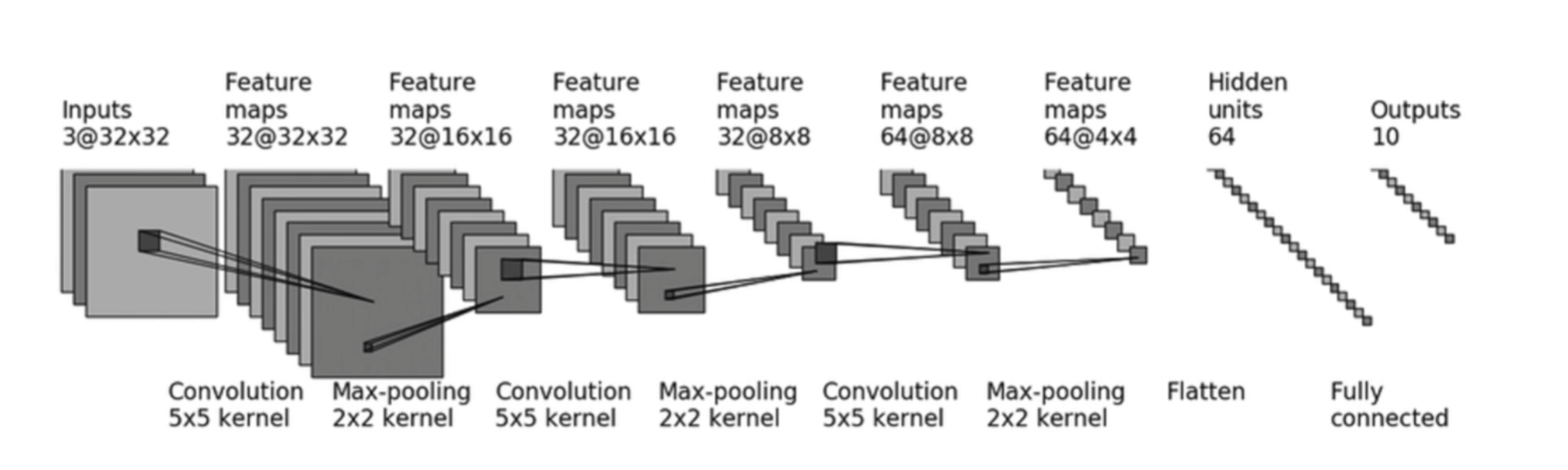
PyTorch in Practice: CIFAR10

• A practical example of a simple classification model targeting the CIFAR10 image dataset.

• First, let’s understand Sequential. nn.Sequential is a special subclass of nn.Module whose purpose is to automatically execute the forward logic. Note: each parameter inside is a class for a certain layer, meaning they must be comma-separated. Sequential simplifies both the model definition and the forward() operation.

 1
 2
 3
 4
 5
 6
 7
 8
 9
10
11
12
13
14
15
16
17
18
19
20
21
22
23
24
25
26
27
28
29
30
31
32
33
34
35
36
37

class CIFAR10_Simple(nn.Module):
    def __init__(self, *args, **kwargs):
        super(CIFAR10_Simple, self).__init__(*args, **kwargs)
        self.conv1 = Conv2d(in_channels=3, out_channels=32, kernel_size=5, padding=2)
        '''
        The value of the padding parameter can be derived from visualizing the image: for a 5x5 convolution kernel, when centered at the image's (0,0), the kernel extends outwards by 2 units. This is a simplified estimation method; in reality, you should substitute values into the dimension formula for calculation (refer to the "Convolution Conv" section).
        '''
        self.model_s = Sequential(
            Conv2d(in_channels=3, out_channels=32, kernel_size=5, padding=2),
            nn.ReLU(),
            MaxPool2d(kernel_size=2),
            Conv2d(in_channels=32, out_channels=32, kernel_size=5, padding=2),
            nn.ReLU(),
            MaxPool2d(2),
            Conv2d(32,64,5,padding=2),
            nn.ReLU(),
            MaxPool2d(2),
            Flatten(),
            Linear(1024, 64),
            nn.ReLU(),
            Linear(64, 10)
        )

    def forward(self, x):
        '''
        x = self.conv1(x)
        x = self.maxpool1(x)
        x = self.conv2(x)
        x = self.maxpool2(x)
        x = self.conv3(x)
        x = self.maxpool3(x)
        x = self.flatten(x)
        x = self.linear1(x)
        x = self.linear2(x)
        '''
        x = self.model_s(x)
        return x

• Before building the model, initially set up DataLoader to handle the dataset.

  • Prepare train_data and test_data independently respectively.

1
2
3
4
5
6

dataset_transfrom = tf.Compose([tf.ToTensor(),tf.Normalize((0.5,0.5,0.5),(0.5,0.5,0.5))])
train_data = torchvision.datasets.CIFAR10("./dataset", transform=dataset_transfrom, download=True)
test_data = torchvision.datasets.CIFAR10("./dataset", train=False, transform=dataset_transfrom, download=True)
# --------
train_loader = DataLoader(dataset=train_data, batch_size=64, shuffle=True, drop_last=True)
test_loader = DataLoader(dataset=test_data, batch_size=64, shuffle=True, drop_last=True)

• After building out the model properly, run a trivial check testing evaluating exactly asserting checking whether output dimension correctly matches expectation guidelines appropriately cleanly.

1
2
3
4
5

cifar = CIFAR10_Simple()
print(cifar)
input = torch.ones((64, 3, 32, 32)) # Test with identical dataset picture sizes
output = cifar(input)
print(output.shape)

• Basic settings before training
  • Define TensorBoard writer
  • Setup device to call the graphics card for accelerated training
  • Instantiate the training model
  • Define the loss function
  • Set up the optimizer

1
2
3
4
5
6

writer = SummaryWriter("./logs")
writer.add_graph(cifar, input)
device = torch.device("cuda" if torch.cuda.is_available() else "cpu")
model = CIFAR10_Simple().to(device)
loss_func = nn.CrossEntropyLoss() # Cross-entropy loss function
optim = torch.optim.SGD(cifar.parameters(), lr=0.01) # Learning rate

• Training section
  • Boilerplate code for the optimizer
  • Record training loss

 1
 2
 3
 4
 5
 6
 7
 8
 9
10
11
12
13
14
15
16

total_step = 0
for epoch in range(10):
    # --- Training section ---
    model.train()
    for data in train_loader:
        imgs, targets = data
        outputs = model(imgs.to(device))
        loss = loss_func(outputs, targets.to(device))
        
        optim.zero_grad()
        loss.backward()
        optim.step()
        
        # Record training loss
        writer.add_scalar("Train_Loss", loss.item(), total_step)
        total_step += 1

• Evaluation section
  • Execute once per epoch
  • with torch.no_grad(): Turn off gradient recording
  • Compile performance metrics

 1
 2
 3
 4
 5
 6
 7
 8
 9
10
11
12
13
14
15
16

model.eval()
    total_test_loss = 0
    total_accuracy = 0
    with torch.no_grad(): # No need to calculate gradients during testing, saves performance
        for data in test_loader:
            imgs, targets = data
            imgs, targets = imgs.to(device), targets.to(device)
            outputs = model(imgs)
            
            # Calculate total loss
            loss = loss_func(outputs, targets)
            total_test_loss += loss.item()
            
            # Calculate accuracy: argmax(1) finds the category index with the highest probability
            accuracy = (outputs.argmax(1) == targets).sum()
            total_accuracy += accuracy

• Visualization

1
2
3
4
5
6
7

# Output to TensorBoard
    writer.add_scalar("Test_Loss", total_test_loss / len(test_loader), epoch)
    writer.add_scalar("Test_Accuracy", total_accuracy / len(test_data), epoch)
    
    print(f"Epoch {epoch+1} finished, Accuracy: {total_accuracy / len(test_data)}")

writer.close()