CS 224n Spring 2024: Assignment #3

a3_spr24_student_handout.pdf

本post从cs224n独立出来，旨在尽可能掌握Assignment3中基于RNN的NMT背后各步的数学原理，以及将代码部分和数学部分对应起来。

参考论文：

NEURAL MACHINE TRANSLATION BY JOINTLY LEARNING TO ALIGN AND TRANSLATE

Neural Machine Translation with RNNs

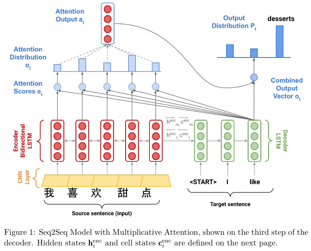
Model description (training procedure)

Given a sentence in the source language, we look up the character or word embeddings from an embeddings matrix, yielding $\mathbf{x}_1, \ldots, \mathbf{x}_m$ ($\mathbf{x}_i \in \mathbb{R}^{e \times 1}$), where $m$ is the length of the source sentence and $e$ is the embedding size.

我们手里的一条源语言句子，由于计算机无法直接理解文字，我们首先要进行“查表”操作，也就是文本中提到的获取词嵌入（look up … embeddings matrix）。假设句子有 $m$ 个词，经过这一步，每个词都被映射成了一个长度为 $e$ 的列向量 $\mathbf{x}_i$。这样一来，整句话就被转换成了一个由实数向量构成的序列

We then feed the embeddings to a convolutional layer$^1$ while maintaining their shapes.

$^1$ : Checkout Convolutional Neural Networks for an in-depth description for convolutional layers if you are not familiar.

带着这些初步的向量表示，模型并没有直接把它们送入主要的编码器，而是先让它们穿过一个卷积层（convolutional layer）。文本中特别强调了这一步“保持了它们的形状”，这意味着经过卷积处理后，我们依然拥有 $m$ 个向量，且每个向量的维度依然是 $e$。这一步的作用通常是对局部的特征进行一次平滑和提取，为后续更深层的语义理解打好基础。

We feed the convolutional layer outputs to the bidirectional encoder, yielding hidden states and cell states for both the forwards ($\rightarrow$) and backwards ($\leftarrow$) LSTMs. The forwards and backwards versions are concatenated to give hidden states $\mathbf{h}_i^{\text{enc}}$ and cell states $\mathbf{c}_i^{\text{enc}}$:

接下来，这些被初步加工过的特征向量正式进入了核心组件——双向编码器（bidirectional encoder）。这里其实包含了两条流水线：一条是前向 LSTM（在数学符号中用向右的箭头 $\rightarrow$ 表示），它顺着我们阅读的习惯，从第一个词读到最后一个词，负责收集每个词左侧的“上文”信息；另一条是后向 LSTM（用向左的箭头 $\leftarrow$ 表示），它逆着顺序，从最后一个词倒着读回来，负责收集每个词右侧的“下文”信息。当这两条流水线各自运转完毕后，对于句子中的任意第 $i$ 个位置，我们就得到了两个不同视角的隐藏状态 $\mathbf{h}_i^{\text{enc}}$ 和细胞状态 $\mathbf{c}_i^{\text{enc}}$，前向( $\overrightarrow{\mathbf{h}_i^{\text{enc}}}$ , $\overrightarrow{\mathbf{c}_i^{\text{enc}}}$ )或后向( $\overleftarrow{\mathbf{h}_i^{\text{enc}}}$ , $\overleftarrow{\mathbf{c}_i^{\text{enc}}}$ )分别的状态量，维度都是 $h \times 1$ 。

$[ ; ]$ 在线性代数中通常表示向量或矩阵的拼接。为了让第 $i$ 个位置最终的表示既包含左侧上下文，又包含右侧上下文，模型将同一时刻 $i$ 的前向状态和后向状态直接“拼接”在一起。因为前向和后向状态都是 $h \times 1$ 的列向量，将它们沿行方向拼接后，最终的联合隐藏状态 $\mathbf{h}_i^{\text{enc}}$ 和联合细胞状态 $\mathbf{c}_i^{\text{enc}}$ 的维度就翻倍了，变成了 $(h+h) \times 1 = \mathbf{2h \times 1}$。

We then initialize the decoder’s first hidden state $\mathbf{h}_0^{\text{dec}}$ and cell state $\mathbf{c}_0^{\text{dec}}$ with a linear projection of the encoder’s final hidden state and final cell state.$^2$

$^2$ : If it’s not obvious, think about why we regard $[\overleftarrow{\mathbf{h}_1^{\text{enc}}} , \overrightarrow{\mathbf{h}_m^{\text{enc}}}]$ as the ‘final hidden state’ of the Encoder.

双向编码器（Encoder）已经工作完毕，看完了整句源语言文本，并在每一个位置都留下了浓缩的上下文信息。接下来的任务就是把这些信息传递给解码器（Decoder），让它开始生成翻译。传递的过程就是通过下面公式中，初始化解码器在第0步的隐藏状态 $\mathbf{h}_0^{\text{dec}}$ 和细胞状态 $\mathbf{c}_0^{\text{dec}}$ 来完成的。解码器的初始状态是从编码器那里继承来的“最终状态”。

编码器在“读完”整句话后的最终状态，可见公式：前向 LSTM 是顺着语序从左到右读的，所以当它读完最后一个词时，它的最终状态自然就落在了句尾，也就是第 $m$ 个位置，记作 $\overrightarrow{\mathbf{h}_m^{\text{enc}}}$。相反，后向 LSTM 是倒着从右向左读的，它“通读全文”后的最后一站其实是句子的开头，也就是第 $1$ 个位置，记作 $\overleftarrow{\mathbf{h}_1^{\text{enc}}}$。

为了把前向和后向这两股贯穿全文的“记忆”汇聚起来，我们按照公式将它们进行了拼接操作 $[\overleftarrow{\mathbf{h}_1^{\text{enc}}} ; \overrightarrow{\mathbf{h}_m^{\text{enc}}}]$。（需注意，在Decoder这一步和公式 (1) (2) 的上下文状态量不一样）

通过这个拼接，我们得到了一个维度为 $2h \times 1$ 的长向量。同样地，对于细胞状态 $\mathbf{c}$，我们用完全相同的逻辑提取出 $[\overleftarrow{\mathbf{c}_1^{\text{enc}}} ; \overrightarrow{\mathbf{c}_m^{\text{enc}}}]$。那么对于 $2h \times 1$ 的向量，我们要将其转换成 $h\times 1$ 才能满足解码器的隐藏层容量。

所以引入权重（投影）矩阵，用来做线性投影(linear projection)，维度是 $h \times 2h$ ，再通过矩阵相乘，映射出 $h\times 1$ 的向量。

With the decoder initialized, we must now feed it a target sentence.

成功初始化了解码器的第 0 步状态（$\mathbf{h}_0^{\text{dec}}$ 和 $\mathbf{c}_0^{\text{dec}}$）之后。现在，解码器已经准备好生成（或在训练时接收）目标语言的句子了。下面内容讲的就是在任意的第 $t$ 步，解码器是如何“吃进”数据并更新自己状态的。

On the $t^{th}$ step, we look up the embedding for the $t^{th}$ subword, $\mathbf{y}_t \in \mathbb{R}^{e \times 1}$.

要让解码器在第 $t$ 步进行工作，我们首先得给它提供当前的输入词，同样需要查表，把目标语言的第 $t$ 个子词（subword）变成一个维度为 $e$ 的词嵌入向量，记作 $\mathbf{y}_t$。

We then concatenate $\mathbf{y}_t$ with the combined-output vector $\mathbf{o}_{t-1} \in \mathbb{R}^{h \times 1}$ from the previous timestep (we will explain what this is later down this page!) to produce $\overline{\mathbf{y}_t} \in \mathbb{R}^{(e+h) \times 1}$.

但是，如果只把 $\mathbf{y}_t$ 喂给解码器，它会缺乏连贯性。为了让解码器知道“我刚才干了什么”，文本中引入了一个非常关键的设计：把当前的词向量 $\mathbf{y}_t$ 与上一步（第 $t-1$ 步）的维度为 $h$ 的联合输出向量 (combined-output vector) $\mathbf{o}_{t-1}$ 拼接在一起，得到新的输入向量 $\overline{\mathbf{y}_t}$，它的维度变成了 $e+h$。

Note that for the first target subword (i.e. the start token) $\mathbf{o}_0$ is a zero-vector. We then feed $\overline{\mathbf{y}_t}$ as input to the decoder.

注意到当 $t=1$ ，也就是解码器刚开始吐出第一个词（或者接收 start token）时，因为前面还没有任何输出，所以初始的 $\mathbf{o}_0$ 就简单地设定为一个全零向量。

关于向Decoder中输入了三个变量后，在LSTM的Decoder里进行了什么计算，需结合CS224N中LSTM的部分进行理解：(generated by Gemini)

• 遗忘门 (Forget Gate)
  • 参与者： 新输入$\overline{\mathbf{y}_t}$和旧的短期记忆$\mathbf{h}_{t-1}^{\text{dec}}$。
  • 动作： 把这两个变量拼接在一起，乘上一个权重矩阵，加上偏置，然后送入一个 Sigmoid 激活函数。
  • 产出： 得到一个介于 0 到 1 之间的向量 $f_t$。
  • 意义： 这个 $f_t$ 会盯着传送带上的旧长期记忆 $\mathbf{c}_{t-1}^{\text{dec}}$ 看。0 代表“彻底忘掉”，1 代表“完全保留”。比如遇到新的主语，它可能就会决定忘掉旧主语的单复数信息。
• 输入门与候选记忆 (Input Gate & Candidate Memory)
  • 参与者： 依然是 $\overline{\mathbf{y}_t}$ 和 $\mathbf{h}_{t-1}^{\text{dec}}$。
  • 动作： 这里分两头行动：
    1. 输入门 $i_t$： 再次经过一个 Sigmoid 函数，产生 0 到 1 的值，决定我们有多希望把新信息存进去。
    2. 候选记忆 $\tilde{\mathbf{c}}_t$： 经过一个 tanh 激活函数，产生 -1 到 1 的值，这代表从当前输入中提取出的全部潜在新知识。
  • 意义： 这两步结合，就是要把提炼出的新知识（$\tilde{\mathbf{c}}_t$）按照我们的渴望程度（$i_t$）进行打包，准备放到传送带上。
• 状态更新 (Cell State Update)
  • 参与者： 旧记忆 $\mathbf{c}_{t-1}^{\text{dec}}$，遗忘门 $f_t$，输入门 $i_t$，候选记忆 $\tilde{\mathbf{c}}_t$。
  • 动作： 纯粹的数学运算。首先用旧记忆乘以遗忘门：$f_t * \mathbf{c}_{t-1}^{\text{dec}}$ （执行“丢弃”动作）；然后加上新的包裹：$i_t * \tilde{\mathbf{c}}_t$ （执行“装载”动作）。
  • 产出： 我们得到了当前时刻的全新细胞状态 $\mathbf{c}_t^{\text{dec}}$。
  • 意义： 长期记忆的传送带在这里完成了向前推进，旧的糟粕被剔除，新的信息被注入。这就是 LSTM 能够跨越长距离保持梯度的核心。
• 输出门与隐藏状态 (Output Gate & Hidden State)
  • 参与者： $\overline{\mathbf{y}_t}$，$\mathbf{h}_{t-1}^{\text{dec}}$，以及刚刚出炉的新细胞状态 $\mathbf{c}_t^{\text{dec}}$。
  • 动作：
    1. 用 $\overline{\mathbf{y}_t}$ 和 $\mathbf{h}_{t-1}^{\text{dec}}$ 经过 Sigmoid 算出一个输出门 $o_t$（决定展示的比例）。
    2. 把刚刚做好的新细胞状态 $\mathbf{c}_t^{\text{dec}}$ 用 tanh 函数“压”到 -1 到 1 之间。
    3. 两者相乘：$\mathbf{h}_t^{\text{dec}} = o_t * \tanh(\mathbf{c}_t^{\text{dec}})$。
  • 产出： 我们得到了当前时刻的全新隐藏状态 $\mathbf{h}_t^{\text{dec}}$。
  • 意义： 细胞状态 $\mathbf{c}_t$ 包含的信息太庞杂了（有些可能是给未来留的伏笔），我们不能全部暴露。输出门 $o_t$ 就像一个滤网，只把当前这一步预测下一个词最需要的那部分特征提取出来，作为对外的公开展示（$\mathbf{h}_t$）。

We then use $\mathbf{h}_t^{\text{dec}}$ to compute multiplicative attention over $\mathbf{h}_1^{\text{enc}}, \dots, \mathbf{h}_m^{\text{enc}}$:

$\mathbf{e}_{t,i}$ is a scalar, the $i$ th element of $\mathbf{e}_t \in \mathbb{R}^{m \times 1}$, computed using the hidden state of the decoder at the $t$ th step, $\mathbf{h}_t^{\text{dec}} \in \mathbb{R}^{h \times 1}$, the attention projection $\mathbf{W}_{\text{attProj}} \in \mathbb{R}^{h \times 2h}$, and the hidden state of the encoder at the $i$ th step, $\mathbf{h}_i^{\text{enc}} \in \mathbb{R}^{2h \times 1}$.

公式(6)是注意力机制的Scoring，解码器现在的状态是 $\mathbf{h}_t^{\text{dec}}$，它需要和字典里的每一个词 $\mathbf{h}_i^{\text{enc}}$进行比对，看看有多匹配。

$(\mathbf{h}_t^{\text{dec}})^T$ , $\mathbf{W}_{\text{attProj}}$ , $\mathbf{h}_i^{\text{enc}}$ 这三者相乘后维度为 $1\times 1$ ，即Scoring出的标量 $\mathbf{e}_{t,i}$ ，它代表了在生成第 $t$ 个翻译词时，源语言句子中第 $i$ 个词的重要程度。 我们把对所有 $m$ 个词的打分收集起来，就得到了一个长度为 $m$ 的得分向量 $\mathbf{e}_t$ 。

为了把公式 (6) 的得分变成标准的“注意力分配比例”，公式 (7) 引入了 softmax 函数。它把向量 $\mathbf{e}_t$ 里的所有数字全部转换为 $0$ 到 $1$ 之间的正数，并且保证它们的总和严格等于 $1$。转换后的结果就是 $\alpha_t$（被称为注意力分布 Attention Distribution）。

公式 (8) 用刚算出来的注意力百分比 $\alpha_{t,i}$，去对字典里的词 $\mathbf{h}_i^{\text{enc}}$ 进行加权求和。把这 $m$ 个按比例缩放的向量全部加起来，我们就得到了最终的注意力输出向量（Attention Output / Context Vector），记作 $\mathbf{a}_t$。 由于被加和的 $\mathbf{h}_i^{\text{enc}}$ 都是 $2h \times 1$ 维的，所以最终得到的 $\mathbf{a}_t$ 也是 $2h \times 1$ 维。

We now concatenate the attention output $\mathbf{a}_t$ with the decoder hidden state $\mathbf{h}_t^{\text{dec}}$ and pass this through a linear layer, tanh, and dropout to attain the combined-output vector $\mathbf{o}_t$.

将注意力输出向量和解码器隐藏状态结合，得到维度为 $3h\times 1$ 的 $u_t$

加入了一个线性投影矩阵 $\mathbf{W}_u$（维度是 $h \times 3h$ ，当它和 $\mathbf{u}_t$ 相乘时，把维度压缩回了标准尺寸 $h \times 1$

首先给它套上一个 tanh 激活函数，将其内部的数值平滑地压缩到 -1 到 1 之间，这赋予了模型非线性的表达能力。紧接着，再让它穿过一层 dropout。dropout 是一种防止模型过拟合的正则化技术，它在训练时会随机屏蔽掉一部分神经元，逼迫模型学到更鲁棒、更泛化的特征。

最后得到联合输出向量(combined-output vector) $\mathbf{o}_t$

Then, we produce a probability distribution $\mathbf{P}_t$ over target subwords at the $t^{th}$ timestep:

我们要把一个 $h$ 维的向量，变成目标语言词典里的一个具体词汇。我们的目标语言词典（Vocabulary）里一共有 $V_t$ 个单词。公式 (12) 引入了一个最终的变换矩阵 $\mathbf{W}_{\text{vocab}}$，它的维度是 $V_t \times h$。相乘后输出一个 $[V_t \times 1]$ 的列向量。这个向量里的每一个数字，就代表了模型对词典里对应单词的“打分”（Logits）。

Here, $V_t$ is the size of the target vocabulary. Finally, to train the network we then compute the cross entropy loss between $\mathbf{P}_t$ and $\mathbf{g}_t$, where $\mathbf{g}_t$ is the one-hot vector of the target subword at timestep $t$:

训练过程使用了交叉熵损失 (Cross Entropy Loss) 函数。简单来说，交叉熵会去对比 $\mathbf{P}_t$ 和 $\mathbf{g}_t$ (one-hot vector)之间的差距。计算出损失 $J_t(\theta)$ 之后，在接下来的代码实现中，模型就会利用反向传播机制，顺着网络一路往回找，去微调那些导致错误的参数 $\theta$。

Implementation and written questions

__init__()

在问题 (c) 的nmt_model.py的__inti__()中，关于神经网络各层的定义，其中self.att_projection的定义需注意，虽然它对应的是 $W_{attProj}$ ，但是在编写代码时，要拆解结合律，决定计算顺序。

应该先算$\mathbf{W}_{\text{attProj}} $ 和 $\mathbf{h}_i^{\text{enc}}$ 相乘，再将其乘积与 $(\mathbf{h}_t^{dec})^T$ 相乘求最终结果，这是因为所有的编码器状态 $\mathbf{h}_i^{\text{enc}}$ 在 Decoder 开始工作前就已经全部计算好了。你可以一次性把整句话的 $\mathbf{h}^{\text{enc}}$ 丢进 Linear 层进行投影（这叫 Pre-computation 预计算）。但是在某一时刻只有一个 $\mathbf{h}_t^{dec}$ 而没有未来的量，导致不能一次性投影完成，而只能把线性层放到了循环中，引发严重的性能问题（虽然数学原理上没错）。下面是一个例子(generated by Gemini) :

假设我们的模型参数如下：

• 隐藏层大小 $h = 512$
• 句子长度 $m = 50$

把 Linear 层塞进循环里

在这个路线里，Linear 层每次要干的活是：把解码器 $1 \times 512$ 的向量，乘以一个 $512 \times 1024$ 的巨大投影矩阵 $\mathbf{W}$。

• 计算量：这需要进行 $512 \times 1024 = \mathbf{524,288}$ 次乘加运算！
• 额外开销：每次循环，PyTorch 都要去内存里把这个包含 50 多万个参数的 $\mathbf{W}$ 矩阵重新搬出来读一遍，并且要经过一层完整的 nn.Linear 封装代码（包含各种维度检查、梯度跟踪的准备）。

然后，算出投影结果后，还得再去和字典做点积：$1 \times 1024$ 的向量乘以 $1024 \times 50$ 的字典，又是 $\mathbf{51,200}$ 次运算。

所以在这个路线下，解码器每走一步，都要背着将近 60万次运算 和一个巨大的矩阵跑。

预计算 + 循环内纯点积

我们把庞大的 Linear 投影放在循环外面，利用 GPU 的超级并行能力，**“一瞬间”**把整本字典从 $50 \times 1024$ 压成了 $50 \times 512$。我们把这本新字典称为 “投影后字典”。

现在我们进入了 for 循环。在第 $t$ 步，我们需要做的乘法是什么呢？

• 计算量：我们直接拿解码器原生的 $1 \times 512$ 向量，去乘以准备好的“投影后字典”（$512 \times 50$）。只需要进行 $512 \times 50 = \mathbf{25,600}$ 次乘加运算！
• 没有额外的层开销：这里不需要调用 nn.Linear，我们在代码里只要写一个极其轻量的纯矩阵乘法指令（比如 torch.matmul 或 @ 符号）就搞定了。不需要加载任何权重矩阵，因为权重矩阵的任务在循环外已经完成了！

encode

问题 (d) 是encoder部分，以及对decoder部分的初始化：

1

self.model_embeddings = ModelEmbeddings(embed_size, vocab)

self.model_embeddings是对ModelEmbeddings的一个实例化，而回到问题 (a) 发现.source是一个nn.Embedding对象：

1
2

self.source = nn.Embedding(num_embeddings=len(vocab.src),embedding_dim=self.embed_size,
                                   padding_idx=src_pad_token_idx)

但是在问题 (a) 中只是对它的实例化，在内存中申请了一个形状为 (num_embeddings, embedding_dim) 的大矩阵。

1

X = self.model_embeddings.source(source_padded)

又因为 nn.Embedding 继承自 nn.Module，而 nn.Module 重写了 __call__ 方法，所以你可以像函数一样使用它（调用），参数设为source_padded这样一个Tensor，它把 Tensor 里的每一个数字当成“行号”，去刚才创建的那个大矩阵里把对应的行找出来，然后输出包含词向量的 Tensor。

下面在将Tensor送进Encoder之前，要用torch.permute变换形状，从(src_len, b, e)变到(b, e, src_len)。那么torch.permute的参数，只是参数位置（索引号）。如下，将原来索引为1的b放到第0个位置，原来索引为2的放到第1个位置，原来索引为0的放到第2个位置。

1

X = X.permute(1, 2, 0)

之后将Tensor X送进LSTM的Encoder后，得到输出：

1
2

output,(last_hidden,last_cell) = self.encoder(X)

output对应的就是双向LSTM的全局上下文向量： $\mathbf{h}_1^{\text{enc}}, \ldots, \mathbf{h}_m^{\text{enc}}$

last_hidden对应的是：$\overrightarrow{\mathbf{h}_m^{\text{enc}}}$ 和 $\overleftarrow{\mathbf{h}_1^{\text{enc}}}$ ，它的形状是 (num_layers * num_directions, batch_size, hidden_size) ，由于它是双向的，所以索引0和索引1分别对应，我们需要将其分离再拼接，形成我们需要的$\overleftarrow{\mathbf{h}_1^{\text{enc}}} ; \overrightarrow{\mathbf{h}_m^{\text{enc}}}$ 。注意torch.cat的参数dim=1表示为横向拼接，即拼接好的向量的列数变成了2 * hidden_size

与投影矩阵相乘的部分，由实例化好的线性层self.h_projection完成。

1

init_decoder_hidden = self.h_projection(torch.cat((last_hidden[0],last_hidden[1]),dim=1))

last_cell同理，不再赘述。

decode

问题 (e) 是decode部分： enc_hiddens_proj = self.att_projection(enc_hiddens) 对应公式 (6) 中 $\mathbf{W}_{\text{attProj}} \mathbf{h}_i^{\text{enc}}$ 的部分。正如在 __init__() 部分讨论的，编码器的全部隐藏状态在进入 decode 时已经固定，所以可以在循环外一次性完成投影预计算，将 enc_hiddens 从 (b, src_len, 2h) 投影为 (b, src_len, h)。

Y = self.model_embeddings.target(target_padded) 和 encode 中对源语言做查表的操作对称，这里调用目标语言的嵌入矩阵，将 target_padded 中的词索引映射成词向量，得到形状为 (tgt_len, b, e) 的张量 Y。

torch.split(Y, 1) 沿第 0 维（时间维度）将 Y 切成一系列 (1, b, e) 的张量。squeeze(Y_t, 0) 去掉多余的维度变为 (b, e)。注意必须指定 dim=0，否则当 batch_size = 1 时会误删 batch 维度。

torch.cat((Y_t, o_prev), dim=1) 对应前文的拼接操作：将 $\mathbf{y}_t$（维度 $e$）与 $\mathbf{o}_{t-1}$（维度 $h$）拼接为 $\overline{\mathbf{y}_t} \in \mathbb{R}^{(e+h)}$。

self.step(...) 内部一次性完成公式 (5)-(11) 的计算：Decoder LSTM 前向传播 → 注意力评分与分布 → 加权求和得到上下文向量 → 线性投影、tanh、dropout，最终产出联合输出向量 $\mathbf{o}_t$。每步将 $\mathbf{o}_t$ 存入列表并更新 o_prev。

torch.stack(combined_outputs, dim=0) 将列表中所有 (b, h) 的张量堆叠为 (tgt_len, b, h)，随后送入公式 (12) 的词汇投影层生成概率分布。

step

问题 (f) 是step部分，即解码器单步计算，内部完成公式 (5)-(11)。核心代码分两段：

第一段（~3行）：Decoder LSTM 前向 + 注意力评分

1
2
3

dec_state = self.decoder(Ybar_t, dec_state)
dec_hidden, dec_cell = dec_state
e_t = torch.bmm(enc_hiddens_proj, torch.unsqueeze(dec_hidden, 2)).squeeze(2)

前两行直接对应公式 (5)：将 $\overline{\mathbf{y}_t}$ 和上一步状态送入 Decoder LSTM，得到新的 dec_state，再拆分为 dec_hidden（$\mathbf{h}_t^{\text{dec}}$）和 dec_cell（$\mathbf{c}_t^{\text{dec}}$），形状均为 (b, h)。

第三行对应公式 (6) 中的注意力评分。这里的关键在于 torch.bmm 的形状要求——它执行批量矩阵乘法，要求输入严格为三维张量 (b, n, m) × (b, m, p) → (b, n, p)。而我们手里的张量：

• enc_hiddens_proj：形状 (b, src_len, h) — 已经是三维，无需处理
• dec_hidden：形状 (b, h) — 只有二维，不满足 bmm 的要求

所以需要 torch.unsqueeze(dec_hidden, 2) 在第 2 维（最后）插入一个维度，将 (b, h) 变为 (b, h, 1)。这样 bmm 的乘法就变成了：

这实质上就是对 batch 内的每一条样本，让 enc_hiddens_proj 的每一行（某个源词的投影）与 dec_hidden 做点积，得到该源词的注意力分数——正是公式 (6) 的 $(\mathbf{h}_t^{\text{dec}})^T \mathbf{W}_{\text{attProj}} \mathbf{h}_i^{\text{enc}}$。

最后 .squeeze(2) 去掉末尾多余的维度 1，从 (b, src_len, 1) 变回 (b, src_len)，得到注意力得分向量 $\mathbf{e}_t$。

第二段（~6行）：注意力加权 → 联合输出

1
2
3
4
5

alpha_t = F.softmax(e_t, dim=1)
a_t = torch.bmm(torch.unsqueeze(alpha_t, 1), enc_hiddens).squeeze(1)
U_t = torch.cat((a_t, dec_hidden), dim=1)
V_t = self.combined_output_projection(U_t)
O_t = self.dropout(torch.tanh(V_t))

F.softmax(e_t, dim=1) 对应公式 (7)，沿 dim=1（即 src_len 维度）做 softmax，将分数归一化为注意力分布 $\alpha_t$，形状仍为 (b, src_len)。

计算上下文向量 $\mathbf{a}_t$（公式 (8)）时又遇到了 bmm 的三维要求。alpha_t 是 (b, src_len)，需要 unsqueeze(alpha_t, 1) 在第 1 维插入，变为 (b, 1, src_len)：

这就是用注意力权重对编码器隐藏状态做加权求和。.squeeze(1) 去掉中间的 1，得到 (b, 2h) 的上下文向量 $\mathbf{a}_t$。

后三行依次对应公式 (9)(10)(11)：torch.cat 拼接 $\mathbf{a}_t$ 与 $\mathbf{h}_t^{\text{dec}}$ 得到 (b, 3h) 的 $\mathbf{u}_t$；线性层投影回 (b, h) 的 $\mathbf{v}_t$；最后 tanh + dropout 得到联合输出 $\mathbf{o}_t$。

Attention Masking

问题 (g) 是关于 step() 中注意力掩码的作用。在 step() 的两段代码之间，有这样一段：

1
2

if enc_masks is not None:
    e_t.data.masked_fill_(enc_masks.bool(), -float('inf'))

enc_masks 由 generate_sent_masks() 生成：它创建一个 (b, src_len) 的零矩阵，然后对 batch 中每条句子，在其实际长度之后的位置全部填 1。换言之，1 标记的是 <pad> token 的位置，0 标记的是真实词的位置。

掩码对注意力计算的影响： masked_fill_ 将 $\mathbf{e}_t$ 中所有对应 <pad> 位置的注意力分数替换为 $-\infty$。当这些 $-\infty$ 的值随后经过 softmax 时，$e^{-\infty} = 0$，因此 <pad> 位置的注意力权重 $\alpha_{t,i}$ 会变为 $0$，而所有真实词的权重之和仍归一化为 $1$。这意味着在公式 (8) 的加权求和中，<pad> 位置的编码器隐藏状态对上下文向量 $\mathbf{a}_t$ 完全没有贡献。

为什么必须这样做： 由于 batch 内各句子长度不一，短句会被 <pad> 填充到统一长度。如果不加掩码，<pad> 对应位置的编码器隐藏状态（本质上是无意义的噪声）会分走一部分注意力权重，从而污染上下文向量，导致翻译质量下降。

Training

问题 (h) 是在代码工作完成后，进入训练阶段。由于我没有海外支付方式，用不了cs224n指定的Google Cloud，所以使用本机显卡进行训练（速度快于文档的预估值）

1

bash run.sh train

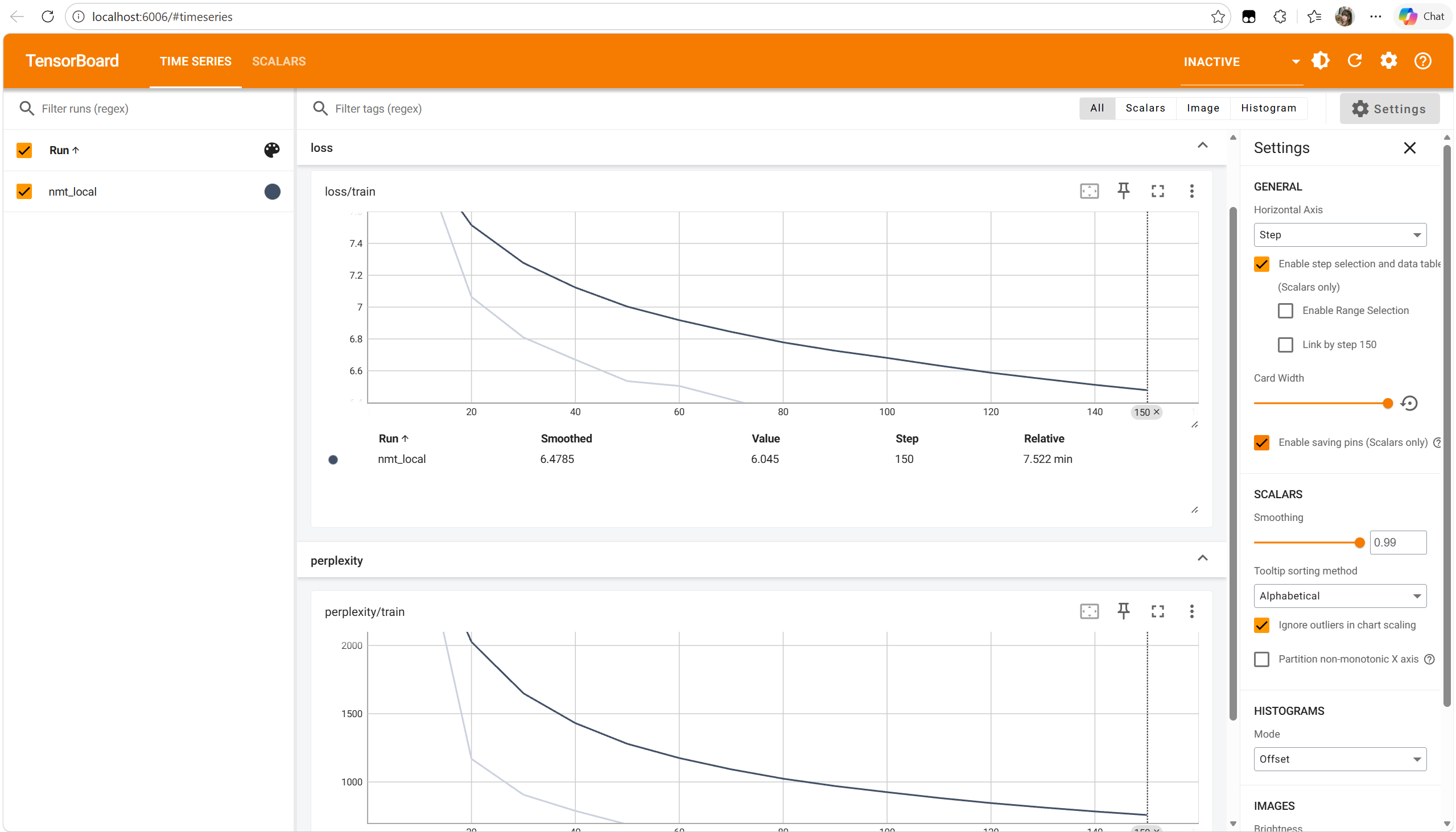
观察tensorboard可见loss曲线并无异常，待训练完成后进行测试评估：

1

bash run.sh test

结果：the model’s corpus BLEU Score is larger than 18, tests passed.

Attention Comparison

最后问题 (i) 是点积注意力、加性注意力分别与乘性注意力进行比较：

Dot Product vs. Multiplicative

• Dot Product Attention: $\mathbf{e}_{t,i} = \mathbf{s}_t^T \mathbf{h}_i$
• Multiplicative Attention: $\mathbf{e}_{t,i} = \mathbf{s}_t^T \mathbf{W} \mathbf{h}_i$

点积注意力的优势：

• 计算速度更快，显存占用更小。 点积注意力没有任何可学习的权重矩阵 $\mathbf{W}$，它仅仅是两个向量的内积。在 GPU 上，这种纯粹的向量点积运算被优化到了极致，没有任何额外的内存开销和参数更新负担。

点积注意力的劣势：

• 强制要求维度严格一致，且表达能力较弱。 要做点积，解码器状态 $\mathbf{s}_t$ 和编码器状态 $\mathbf{h}_i$ 的维度必须完全相同。更致命的是，它假设这两个空间天然就是对齐的。而乘性注意力多了一个矩阵 $\mathbf{W}$，不仅允许两者的维度不同（$\mathbf{W}$ 可以做维度转换），还能通过学习 $\mathbf{W}$ 将它们投影到一个更好的共享特征空间中再进行比较。

Additive vs. Multiplicative

• Additive Attention: $\mathbf{e}_{t,i} = \mathbf{v}^T \tanh(\mathbf{W}_1 \mathbf{h}_i + \mathbf{W}_2 \mathbf{s}_t)$
• Multiplicative Attention: $\mathbf{e}_{t,i} = \mathbf{s}_t^T \mathbf{W} \mathbf{h}_i$

(注：Additive Attention 也就是大名鼎鼎的 Bahdanau Attention，它是 Attention 机制的开山鼻祖；而 Multiplicative 则是 Luong Attention 的核心。)

加性注意力的优势：

• 在特征维度很大时，表现通常更好（模型容量大）。 乘性注意力在维度很大时，点积的结果方差会变得极其巨大，容易把 Softmax 推向梯度消失的边缘（也就是后来 Transformer 引入缩放因子的原因）。而加性注意力通过 $\tanh$ 激活函数将内部数值稳稳地压制在 $[-1, 1]$ 之间，天然具有极好的数值稳定性，对超大维度的宽容度更高。

加性注意力的劣势：

• 计算效率较低，难以发挥底层矩阵乘法的极致加速。 乘性注意力可以极其优雅地打包成一个巨大的矩阵乘法（在 Transformer 里就是 $\mathbf{Q}\mathbf{K}^T$），这正是现代 GPU 最擅长的事情。而加性注意力不仅要做两次独立的线性变换，还要过一遍非线性激活函数 $\tanh$，最后再乘一个向量 $\mathbf{v}$。这种复杂的计算图打破了矩阵乘法的纯粹性，导致它在实际工程中的运行速度明显慢于乘性注意力。

Analyzing NMT Systems

问题 (a) 是为什么在embedding层后加1D卷积后，再输入双向encoder效果会好一些？

添加一维卷积层可以作为 n-gram 特征提取器，用于捕捉局部组合性。由于中文词语通常由多个词素组成（例如，“电”+“脑”=“电脑”），一维卷积神经网络的滑动窗口会在序列建模之前，将相邻字符/子词的嵌入向量显式地组合成更高层次的语义表示（一个词或短语）。这提供了一种层级结构，其中卷积神经网络处理局部词汇语义（充当软分词器），从而使双向编码器能够专注于学习全局的、长程的句法依存关系。

问题 (b) 是分析四句中文为什么翻译错了，那么作为普通话母语者不难解答：

i. (2 points) Source Sentence: 贼人其后被警方拘捕及被判处盗窃罪名成立。 Reference Translation: the culprits were subsequently arrested and convicted. NMT Translation: the culprit was subsequently arrested and sentenced to theft.

ii. (2 points) Source Sentence: 几乎已经没有地方容纳这些人, 资源已经用尽。 Reference Translation: there is almost no space to accommodate these people, and resources have run out. NMT Translation: the resources have been exhausted and resources have been exhausted.

iii. (2 points) Source Sentence: 当局已经宣布今天是国殇日。 Reference Translation: authorities have announced a national mourning today. NMT Translation: the administration has announced today’s day. NMT Translation: the administration has announced today’s day.

iv. (2 points) Source Sentence: 俗语有云:“唔做唔错”。 Reference Translation: “ act not, err not ”, so a saying goes. NMT Translation: as the saying goes, “ it’s not wrong. ”

• (i) 是单/复数的问题，缺少上下文以及整体理解，难以判断“贼人”是复数还是单数。
• (ii) “资源已经用尽”被重复翻译了两遍，简单来说是注意力先偏移到了后半句，然后NMT不知道前半句没有翻译，加上前面错译出的"…and"，导致重复翻译后半句。
• (iii) src.vocab没有记录“国殇”，所以NMT越过了这个词。
• (iv) 本质是句俗语，或者说是粤语，而多数模型都是基于普通话训练的。

BLEU

BLEU score is the most commonly used automatic evaluation metric for NMT systems. It is usually calculated across the entire test set, but here we will consider BLEU defined for a single example. Suppose we have a source sentence s, a set of k reference translations $\mathbf{r}_1,\dots,\mathbf{r}_k$, and a candidate translation c. To compute the BLEU score of c, we first compute the modified n-gram precision pn of c, for each of n = 1,2,3,4, where n is the n in n-gram:

BLEU 分数是 NMT (神经机器翻译) 系统中最常用的自动评估指标。它通常在整个测试集上计算，但在这里我们将考虑为单个示例定义的 BLEU。假设我们有一个源句子 $\mathbf{s}$，一组 $k$ 个参考翻译 $\mathbf{r}_1,\dots,\mathbf{r}_k$，以及一个候选翻译 $\mathbf{c}$。为了计算 $\mathbf{c}$ 的 BLEU 分数，我们首先计算 $\mathbf{c}$ 的修正 n-gram 精确度 (modified n-gram precision) $p_n$，其中 $n = 1, 2, 3, 4$，$n$ 是 n-gram 中的 $n$：

Here, for each of the n-grams that appear in the candidate translation c, we count the maxi mum number of times it appears in any one reference translation, capped by the number of times it appears in c (this is the numerator). We divide this by the number of n-grams in c (denominator).

这里，对于出现在候选翻译 $\mathbf{c}$ 中的每一个 $n$-gram，我们计算它在任何一个参考翻译中出现的最大次数，上限为它在 $\mathbf{c}$ 中出现的次数（这是分子）。我们将其除以 $\mathbf{c}$ 中 $n$-gram 的数量（分母）。

$p_n$ 公式的分母部分比较清晰，分子部分我们继续拆解：

$\text{Count}_{\mathbf{c}}(\text{ngram})$ : 该词组在模型输出中出现几次。

$\max_{i=1,\dots,k} \text{Count}_{\mathbf{r}_i}(\text{ngram})$ : 该词组在所有参考答案中出现次数最多的那一次。比如三个参考答案里，the 分别出现了 1、2、1 次，那么这个值就是 2。

$\min(\dots)$ : 这是**截断（Clipping）**机制。它规定：即便你在输出里写了 10 个 the，如果参考答案里最多只出现了 2 个，那我也只算你命中了 2 个。

综上，公式可以被翻译成：

$$ > p_n = \frac{\text{被认可的 n-gram 匹配总数}}{\text{候选翻译中总共生成的 n-gram 数量}} > $$

Next, we compute the brevity penalty BP. Let $len(\mathbf{c})$ be the length of c and let $len(\mathbf{r})$ be the length of the reference translation that is closest to $len(\mathbf{c})$ (in the case of two equally-close reference translation lengths, choose $len(\mathbf{r})$ as the shorter one).

接下来，我们计算长度惩罚 (brevity penalty) $BP$。令 $len(\mathbf{c})$ 为 $\mathbf{c}$ 的长度，令 $len(\mathbf{r})$ 为最接近 $len(\mathbf{c})$ 的参考翻译的长度（在有两个同样接近的参考翻译长度的情况下，选择较短的那个作为 $len(\mathbf{r})$）。

那么引入 $BP$ 有什么用？首先 $len(\mathbf{c}) \geq len(\mathbf{r})$ 时 $BP=1$ ，这是在NMT输出较长时，$BP$ 不需要惩罚它，而会在 $p_n$ 的分母体现（分母变大，概率降低）。

$len(\mathbf{c}) < len(\mathbf{r})$ 时引入指数惩罚，如果NMT只翻译最有把握的一个词（比如输出一个单词 apple），$p_n$ 可能是 100%，但这没有意义。这个指数函数 $\exp(1 - r/c)$ 在 $c$ 越小时，值会迅速接近 0，从而给短句一个沉重的打击。

Lastly, the BLEU score for candidate c with respect to $\mathbf{r}_1,\dots,\mathbf{r}_k$ is:

最后，候选 $\mathbf{c}$ 相对于 $\mathbf{r}_1,\dots,\mathbf{r}_k$ 的 BLEU 分数为：

本质上等同于：

$$ > BLEU = BP \times (p_1^{\lambda_1} \cdot p_2^{\lambda_2} \cdot p_3^{\lambda_3} \cdot p_4^{\lambda_4}) > $$

where $\lambda_1, \lambda_2, \lambda_3, \lambda_4$ are weights that sum to 1. The log here is natural log.

其中 $\lambda_1, \lambda_2, \lambda_3, \lambda_4$ 是总和为 1 的权重。此处的 $\log$ 是自然对数。

几何平均的一个特性是：如果其中任何一项 $p_n$ 为 0，最终结果就会是 0。所以模型的词汇和语序的正确性都会被计算。

问题 (c) 结合实例运算：

i. Source Sentence s: 需要有充足和可预测的资源。 Reference Translation $r_1$ : resources have to be sufficient and they have to be predictable Reference Translation $r_2$ : adequate and predictable resources are required NMT Translation $c_1$ : there is a need for adequate and predictable resources NMT Translation $c_2$ : resources be sufficient and predictable to Please compute the BLEU scores for and $c_1$ $c_2$. Let $\lambda_i = 0.5$ for $i \in \{1, 2\}$ and $\lambda_i = 0$ for $i \in \{3, 4\}$ (this means we ignore 3-grams and 4-grams, i.e., don’t compute $p_3$ or $p_4$). When computing BLEU scores, show your work (i.e., show your computed values for $p_1$, $p_2$, $len(c)$, $len(r)$ and $BP$). Note that the BLEU scores can be expressed between 0 and 1 or between 0 and 100. The code is using the 0 to 100 scale while in this question we are using the 0 to 1 scale. Please round your responses to 3 decimal places.

先计算 $c_1$ : $len(c_1)=9$ 更接近于 $len(r_1)=11$ , $BP=exp(1-\frac{11}{9})$

$p_1$ 匹配的Unigrams 为 {adequate, and, predictable, resources}，共 4 个。 $p_1=4/9$

$p_2$ 匹配的Bigrams 为 {adequate and, and predictable, predictable resources}，共 3 个。 $p_2=3/8$

$BLEU_{c1} = BP \times \sqrt{p_1 \times p_2}$

$c_2$ 同理。

ii. Our hard drive was corrupted and we lost Reference Translation $r_1$. Please recom pute BLEU scores for $c_1$ and $c_2$, this time with respect to $r_2$ only. Which of the two NMT translations now receives the higher BLEU score? Do you agree that it is the better translation?

计算方式不变，但是在去掉了 $r_1$ 后， ${BLEU}_{c_1}$ 不变， ${BLEU}_{c_2}$ 大幅缩小（由于 $p_1$ 和 $p_2$ 下降）

这说明了 $c_1$ 的鲁棒性更强，它使用了更通用的词汇（如 adequate），即使在参考答案有限的情况下，依然能保持较合理的得分，这更符合人类对“好翻译”的评价标准。

iv. List two advantages and two disadvantages of BLEU, compared to human evaluation, as an evaluation metric for Machine Translation.

优点不列了，缺点：BLEU 仅进行字面上的 N-gram 匹配，缺乏语义理解。由于 BLEU 主要关注局部词汇的重合度，它往往无法识别严重的语法错误或逻辑扭曲。一个逻辑完全相反、但在词汇上高度重合的句子可能获得极高的 BLEU 分，却无法被人类理解，所以它无法准确衡量语言质量。

问题 (d) 是Beam Search相关的，关于训练次数与其“假设”质量的问题，比如i. 要求进行三个对比：

 1
 2
 3
 4
 5
 6
 7
 8
 9
10
11
12
13
14
15
16
17
18
19
20
21
22

// iteration 200
{
            "hypothesis": [
                "▁it",
                "▁is",
                "▁not",
                "▁that",
                "▁the",
                "▁united",
                "▁nations",
                "▁of",
                "▁the",
                "▁united",
                "▁nations",
                "▁of",
                "▁the",
                "▁united",
                "▁nations",
                "."
            ],
            "score": -31.211565017700195
        }

 1
 2
 3
 4
 5
 6
 7
 8
 9
10
11
12
13
14
15
16
17
18
19
20

// iteration 3000
{
            "hypothesis": [
                "▁i",
                "▁would",
                "▁also",
                "▁like",
                "▁to",
                "▁clarify",
                "▁the",
                "▁number",
                "▁of",
                "▁cases",
                "▁in",
                "▁the",
                "▁conference",
                "."
            ],
            "score": -15.013087272644043
        }

 1
 2
 3
 4
 5
 6
 7
 8
 9
10
11
12
13
14
15
16
17
18
19

// iteration 17200 (last)
{
            "hypothesis": [
                "▁i",
                "▁have",
                "▁also",
                "▁clarified",
                "▁a",
                "▁number",
                "▁of",
                "▁matters",
                "▁raised",
                "▁by",
                "▁the",
                "▁conference",
                "."
            ],
            "score": -7.69414758682251
        }